Setting the Scene

Overview

Teaching: 5 min
Exercises: 0 min

Questions

• What are we teaching in this course?

• What motivated the selection of topics covered in the course?

Objectives

• Setting the scene and expectations

• Making sure everyone has all the necessary software installed

Introduction

So, you have gained basic software development skills either by self-learning or attending, e.g., a novice Software Carpentry course. You have been applying those skills for a while by writing code to help with your work and you feel comfortable developing code and troubleshooting problems. However, your software has now reached a point where it is spread across multiple Notebooks with hundreds of cells in each. Perhaps it’s involving more researchers (developers) and users, and more collaborative development effort is needed to add new functionality while ensuring previous development efforts remain functional and maintainable.

This course provides an intro into skills and practices to help you restructure existing code and design more robust, reusable, readable and maintainable code.

Section 1: Setting up Software Environment

In the first section we are going to set up our working environment and familiarise ourselves with various tools and techniques for software development in a typical collaborative code development cycle:

• Virtual environments for isolating a project from other projects developed on the same machine
• Command line for running code and interacting with the command line tool Git,
• Integrated Development Environment for code development, testing and debugging, and
• Python code style guidelines to make sure our code is documented, readable and consistently formatted.

Before We Start

A few notes before we start.

Prerequisite Knowledge

This is an intermediate-level software development course intended for people who have already been developing code in Python (or other languages) and applying it to their own problems after gaining basic software development skills. So, it is expected for you to have some prerequisite knowledge on the topics covered, as outlined at the beginning of the lesson.

Setup, Common Issues & Fixes

Have you setup and installed all the tools and accounts required for this course? Check the list of common issues, fixes & tips if you experience any problems running any of the tools you installed - your issue may be solved there.

Compulsory and Optional Exercises

Exercises are a crucial part of this course and the narrative. They are used to reinforce the points taught and give you an opportunity to practice things on your own. Please do not be tempted to skip exercises as that will get your local software project out of sync with the course and break the narrative. Exercises that are clearly marked as “optional” can be skipped without breaking things but we advise you to go through them too, if time allows. All exercises contain solutions but, wherever possible, try and work out a solution on your own.

Outdated Screenshots

Throughout this lesson we will make use and show content from Graphical User Interface (GUI) tools (Jupyter Lab and GitHub). These are evolving tools and platforms, always adding new features and new visual elements. Screenshots in the lesson may then become out-of-sync, refer to or show content that no longer exists or is different to what you see on your machine. If during the lesson you find screenshots that no longer match what you see or have a big discrepancy with what you see, please open an issue describing what you see and how it differs from the lesson content. Feel free to add as many screenshots as necessary to clarify the issue.

Let Us Know About the Issues

The original materials were adapted specifically for this workshop. They weren’t used before, and it is possible that they contain typos, code errors, or underexplained or unclear moments. Please, let us know about these issues. It will help us to improve the materials and make the next workshop better.

Key Points

• This lesson focuses on core tools and practices for keeping your Jupyter Notebooks readable and maintainable.

• The lesson follows on from the novice Software Carpentry lesson, but this is not a prerequisite for attending as long as you have some basic Python and command line skills, and you have been using them for a while writing code to help with your work.

Section 1: Setting Up Environment For Collaborative Code Development

Overview

Teaching: 5 min
Exercises: 0 min

Questions

• What tools are needed to collaborate on code development effectively?

Objectives

• Provide an overview of all the different tools that will be used in this course.

The first section of the course is dedicated to setting up your environment for collaborative software development and introducing the project that we will be working on throughout the course. In order to build working (research) software efficiently and to do it in collaboration with others rather than in isolation, you will have to get comfortable with using a number of different tools interchangeably as they’ll make your life a lot easier. There are many options when it comes to deciding which software development tools to use for your daily tasks - we will use a few of them in this course that we believe make a difference. There are sometimes multiple tools for the job - we select one to use but mention alternatives too. As you get more comfortable with different tools and their alternatives, you will select the one that is right for you based on your personal preferences or based on what your collaborators are using.

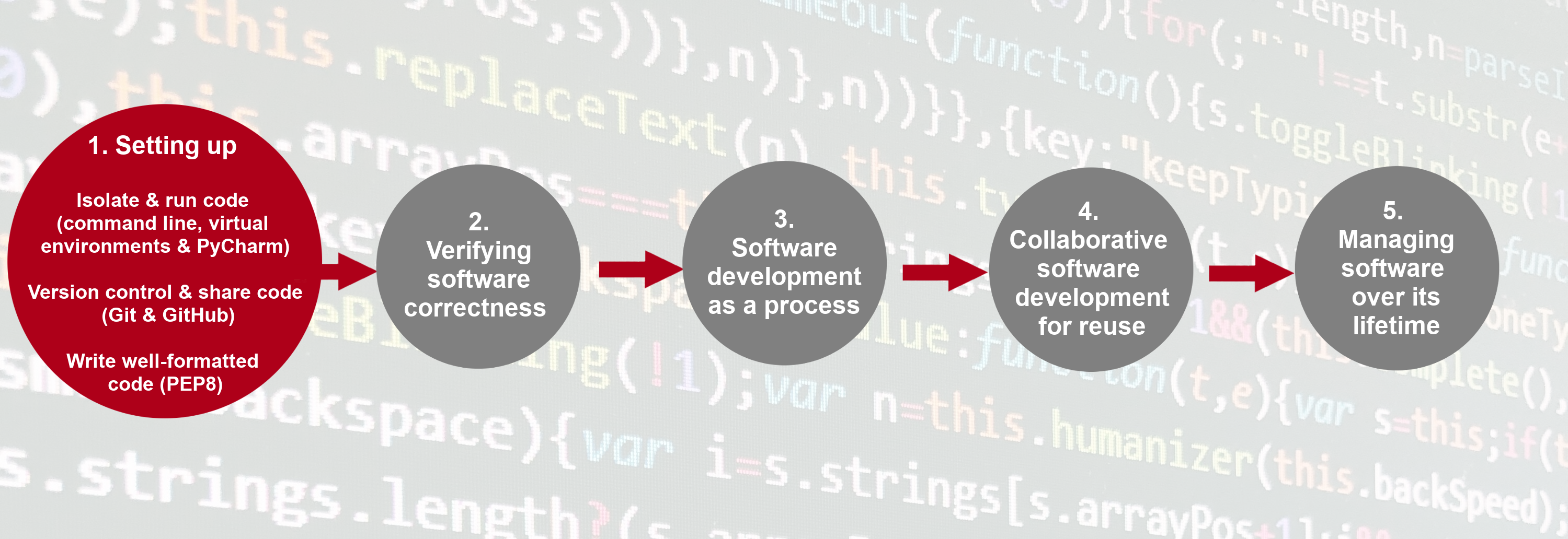
Here is an overview of the tools we will be using.

Setup, Common Issues & Fixes

Have you setup and installed all the tools and accounts required for this course? Check the list of common issues, fixes & tips if you experience any problems running any of the tools you installed - your issue may be solved there.

Command Line & Python Virtual Development Environment

We will use the command line (also known as the command line shell/prompt/console) to run our Python code and interact with the version control tool Git and software sharing platform GitHub. We will also use command line tools venv and pip to set up a Python virtual development environment and isolate our software project from other Python projects we may work on.

Note: some Windows users experience the issue where Python hangs from Git Bash (i.e. typing python causes it to just hang with no error message or output) - see the solution to this issue.

Integrated Development Environment (IDE)

An IDE integrates a number of tools that we need to develop a software project that goes beyond a single script - including a smart code editor, a code compiler/interpreter, a debugger, etc. It will help you write well-formatted and readable code that conforms to code style guides (such as PEP8 for Python) more efficiently by giving relevant and intelligent suggestions for code completion and refactoring. IDEs often integrate command line console and version control tools - we teach them separately in this course as this knowledge can be ported to other programming languages and command line tools you may use in the future (but is applicable to the integrated versions too).

There are several popular IDEs for Python, such as IDLE, PyCharm, Spyder, VS Studio, and so on. In this course, we will use Jupyter Lab - a free, open-source IDE, widely used in the astronomic community.

Is JupyterLab actually an IDE?

JupyterLab is the next evolutionary step for the Jupyter Notebooks, a web-based interactive environment for exploratory coding. While Jupyter Notebooks lack some of the features of classical IDEs (most notably, a debugger), the latest versions of JupyterLab include all the necessary functionality. Terminology aside, JupyterLab is a very popular tool for data analysis and in the research community. More so, JupyterLab still bears a strong resemblance to Jupyter Notebooks, Google Colab and LSST Rubin Science Platform (RSP) Notebook aspect. Many astronomical platforms that provide access to computational resources and observational datasets also have Jupyter Notebooks installed. For this reason, in this course, we aim to show which tools and practices can help you write high-quality, reusable, and reliable software using JupyterLab. The original version of this course was developed for PyCharm IDE, which is usually considered to be more suited for software development that is not related to data exploration and analysis. That course is included in the Carpentries Incubator program, and you can access it here.

Python Coding Style

Most programming languages will have associated standards and conventions for how the source code should be formatted and styled. Although this sounds pedantic, it is important for maintaining the consistency and readability of code across a project. Therefore, one should be aware of these guidelines and adhere to whatever the project you are working on has specified. In Python, we will be looking at a convention called PEP8.

Let’s get started with setting up our software development environment!

Key Points

• In order to develop (write, test, debug, backup) code efficiently, you need to use a number of different tools.

• When there is a choice of tools for a task you will have to decide which tool is right for you, which may be a matter of personal preference or what the team or community you belong to is using.

Introduction to Our Software Project

Overview

Teaching: 10 min
Exercises: 0 min

Questions

• What is the design architecture of our example software project?

• Why is splitting code into smaller functional units (modules) good when designing software?

Objectives

• Use Git to obtain a working copy of our software project from GitHub.

• Inspect the structure and architecture of our software project.

• Understand Model-View-Controller (MVC) architecture in software design and its use in our project.

Light Curve Analysis Project

For this workshop, let’s assume that you have joined a software development team that has been working on the light curve analysis project developed in Python and stored on GitHub. The purpose of this software is to analyze the variability of astronomical sources, using observations that come from different instruments.

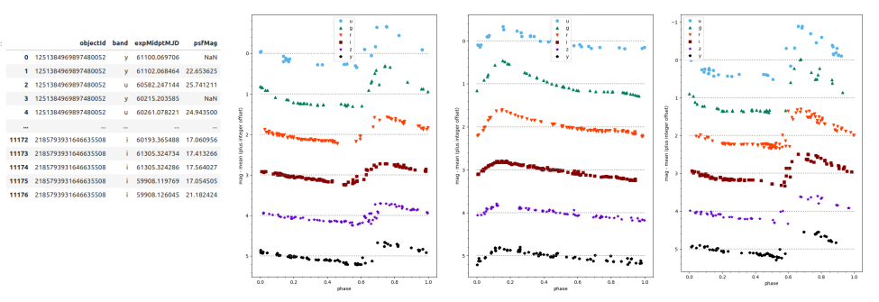
What Does Light Curve Dataset Contain?

For developing and testing our software project, we will use two RR Lyrae candidates variability datasets.

The first dataset, kepler_RRLyr.csv, contains observations coming from the Kepler space telescope. In this dataset, all observations are related to the same source, i.e. the whole table represents a single light curve. The second dataset, lsst_RRLyr.pkl, contains synthetic observations of 25 presumably variable sources from the LSST Data Preview 0. Considering that the datasets come from different instruments, they also have different formats and column names - a common situation in real life. It is always a good idea to develop your software in such a way that it remains usable even if the format of the input data has changed. We will use the differences of the datasets to illustrate some of the topics during this workshop.

The project is not finished and contains some errors. You will be working on your own and in collaboration with others to fix and build on top of the existing code during the course.

Downloading Our Software Project

To start working on the project, you will first create a copy of the software project template repository from GitHub within your own GitHub account and then obtain a local copy of that project (from your GitHub) on your machine.

1. Make sure you have a GitHub account and that you have set up your SSH key pair for authentication with GitHub, as explained in Setup.
2. Log into your GitHub account.

3. Go to the software project repository in GitHub.

   

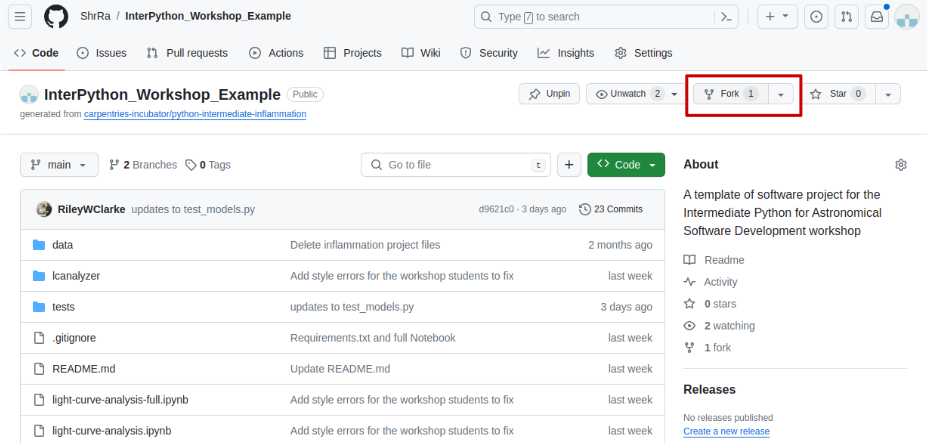
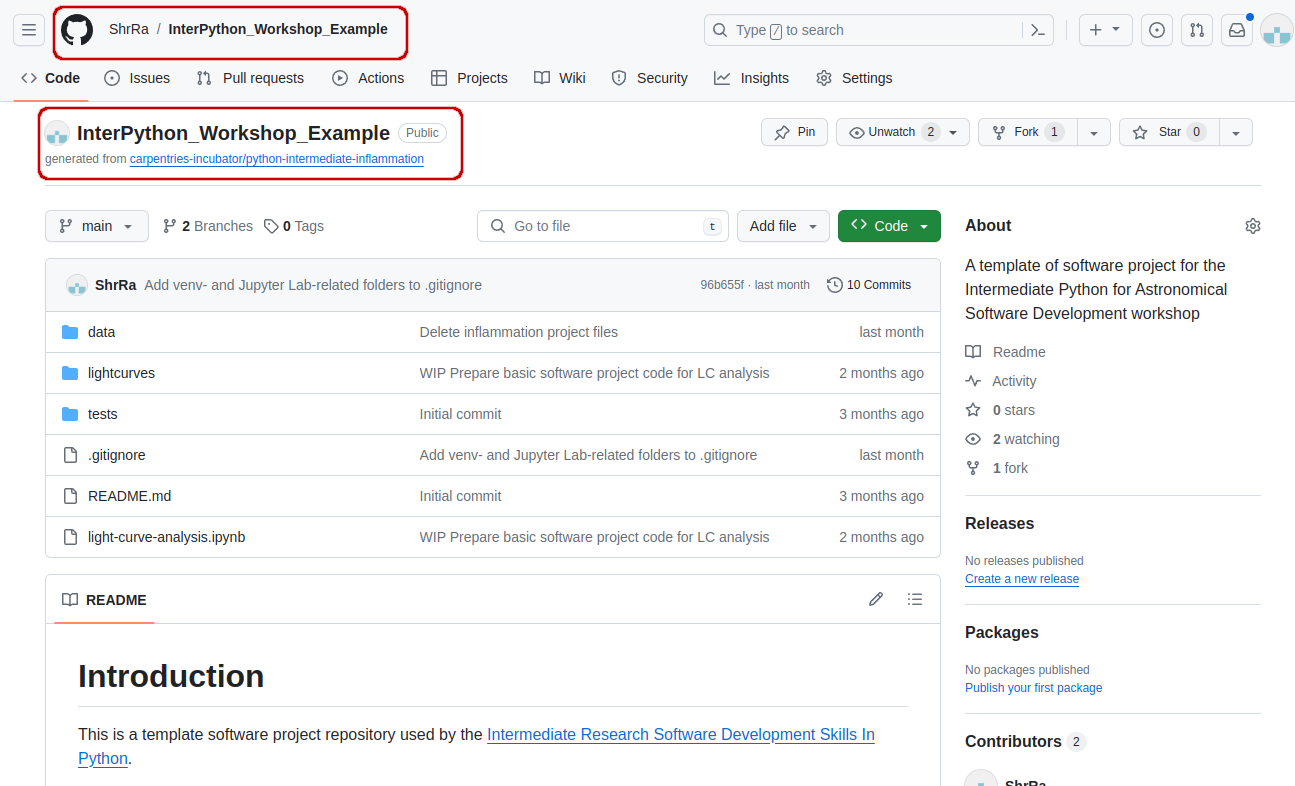
4. Click the Fork button towards the top right of the repository’s GitHub page to create a fork of the repository under your GitHub account. Remember, you will need to be signed into GitHub for the Fork button to work.

   Note: each participant is creating their own fork of the project to work on.

5. Make sure to select your personal account and set the name of the project to InterPython_Workshop_Example (you can call it anything you like, but it may be easier for future group exercises if everyone uses the same name). Also set the new repository’s visibility to ‘Public’ - so it can be seen by others and by third-party Continuous Integration (CI) services (to be covered later on in the course) and select the Copy the main branch only checkbox.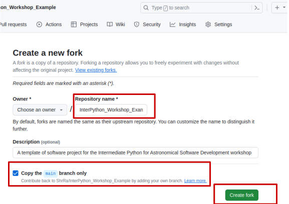

   

6. Click the Create fork button and wait for GitHub to import the copy of the repository under your account.

7. Locate the forked repository under your own GitHub account. GitHub should redirect you there automatically after creating the fork. If this does not happen, click your user icon in the top right corner and select Your Repositories from the drop-down menu, then locate your newly created fork.

   

Exercise: Obtain the Software Project Locally

Using the command line, clone the copied repository from your GitHub account into the home directory on your computer using SSH. Which command(s) would you use to get a detailed list of contents of the directory you have just cloned?

Solution

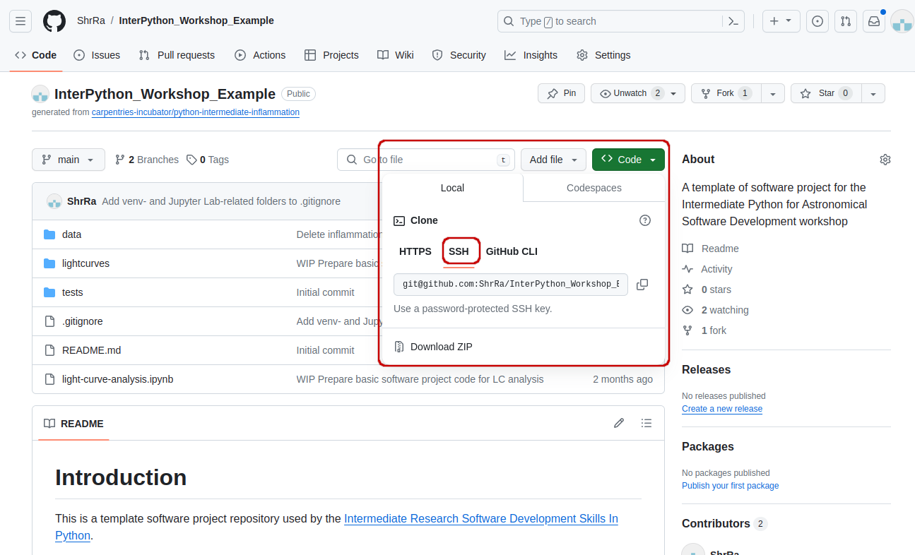
1. Find the SSH URL of the software project repository to clone from your GitHub account. Make sure you do not clone the original template repository but rather your own copy, as you should be able to push commits to it later on. Also make sure you select the SSH tab and not the HTTPS one. These two protocols implement different security measures, and since 2021 GitHub offers full support only for the SSH cloning; namely, you won’t be able to send your changes to the repository if you use HTTPS method.

1. Make sure you are located in your home directory in the command line with:

    $ cd ~
   

2. From your home directory in the command line, do:

    $ git clone git@github.com:<YOUR_GITHUB_USERNAME>/InterPython_Workshop_Example.git
   

   Make sure you are cloning your copy of the software project and not the template repository.

3. Navigate into the cloned repository folder in your command line with:

    $ cd InterPython_Workshop_Example
   

   Note: If you have accidentally copied the HTTPS URL of your repository instead of the SSH one, you can easily fix that from your project folder in the command line with:

    $ git remote set-url origin git@github.com:<YOUR_GITHUB_USERNAME>/InterPython_Workshop_Example.git
   

Our Software Project Structure

Let’s inspect the content of the software project from the command line. From the root directory of the project, you can use the command ls -l to get a more detailed list of the contents. You should see something similar to the following.

$ cd ~/InterPython_Workshop_Example
$ ls -l
total 284
drwxrwxr-x 2 alex alex     52 Jan 10 20:29 data
-rw-rw-r-- 1 alex alex 285218 Jan 10 20:29 light-curve-analysis.ipynb
drwxrwxr-x 2 alex alex     58 Jan 10 20:29 lcanalyzer
-rw-rw-r-- 1 alex alex   1171 Jan 10 20:29 README.md
drwxrwxr-x 2 alex alex     51 Jan 10 20:29 tests
...

As can be seen from the above, our software project contains the README file (that typically describes the project, its usage, installation, authors and how to contribute), Jupyter Notebook light-curve-analysis.ipynb, and three directories - lcanalyzer, data and tests.

The Jupyter Notebook light-curve-analysis.ipynb is where exploratory analysis is done, and on closer inspection, we can see that the lcanalyzer directory contains two Python scripts - views.py and models.py. We will have a more detailed look into these shortly.

$ cd ~/InterPython_Workshop_Example/lcanalyzer
$ ls -l
total 12
-rw-rw-r-- 1 alex alex 903 Jan 10 20:29 models.py
-rw-rw-r-- 1 alex alex 718 Jan 10 20:29 views.py
...

Directory data contains three files with the lightcurves coming from two instruments, Kepler and LSST:

$ cd ~/InterPython_Workshop_Example/data
$ ls -l
total 24008
-rw-rw-r-- 1 alex alex 23686283 Jan 10 20:29 kepler_RRLyr.csv
-rw-rw-r-- 1 alex alex   895553 Jan 10 20:29 lsst_RRLyr.pkl
-rw-rw-r-- 1 alex alex   895553 Jan 10 20:29 lsst_RRLyr_protocol_4.pkl
...

The lsst_RRLyr_protocol_4.pkl file contains the same data as lsst_RRLyr.pkl, but it’s saved using an older data protocol, compatible with older versions of the packages we’ll be using.

Exercise: Have a Peek at the Data

Which command(s) would you use to list the contents or a first few lines of data/kepler_RRLyr.csv file?

Solution

1. To list the entire content of a file from the project root do: cat data/kepler_RRLyr.csv.
2. To list the first 5 lines of a file from the project root do: head -n 5 data/kepler_RRLyr.csv.

time,flux,flux_err,quality,timecorr,centroid_col,centroid_row,cadenceno,sap_flux,sap_flux_err,sap_bkg,sap_bkg_err,pdcsap_flux,pdcsap_flux_err,sap_quality,psf_centr1,psf_centr1_err,psf_centr2,psf_centr2_err,mom_centr1,mom_centr1_err,mom_centr2,mom_centr2_err,pos_corr1,pos_corr2
...

Pay attention that while the .csv format is human-readable, if you try to run head -n 5 data/lsst_RRLyr.pkl, the output will be non-human-readable.

Directory tests contains several unit tests - during this workshop we are not going to touch this topic, but you are welcome to look at the Testing workshop to learn how these tests are written, how they contribute to the robustness of your software and how to automatize their execution.

$ ls -l tests
total 8
-rw-rw-r-- 1 alex alex 941 Jan 10 20:29 test_models.py
...

An important thing to note here is that the structure of the project is not arbitrary. One of the big differences between novice and intermediate software development is planning the structure of your code. This structure includes software components and behavioural interactions between them (including how these components are laid out in a directory and file structure). A novice will often make up the structure of their code as they go along. However, for more advanced software development, we need to plan this structure - called a software architecture - beforehand.

Let’s have a more detailed look into what a software architecture is and which architecture is used by our software project before we start adding more code to it.

Software Architecture

A software architecture is the fundamental structure of a software system that is decided at the beginning of project development based on its requirements and cannot be changed that easily once implemented. It refers to a “bigger picture” of a software system that describes high-level components (modules) of the system and how they interact.

In software design and development, large systems or programs are often decomposed into a set of smaller modules each with a subset of functionality. Typical examples of modules in programming are software libraries; some software libraries, such as numpy and matplotlib in Python, are bigger modules that contain several smaller sub-modules. Another example of modules are classes in object-oriented programming languages.

There are various software architectures around defining different ways of dividing the code into smaller modules with well defined roles. In this project, we use Model-View-Controller (MVC) Architecture that divides the program logic into three interconnected modules:

• Model (data)
• View (client interface), and
• Controller (processes that handle input/output and manipulate the data).

Model represents the data used by a program and also contains operations/rules for manipulating and changing the data in the model. This may be a database, a file, a single data object or a series of objects - for example a table representing light curve observations.

View is the means of displaying data to users/clients within an application (i.e. provides visualisation of the state of the model). For example, displaying a window with input fields and buttons (Graphical User Interface, GUI) or textual options within a command line (Command Line Interface, CLI) are examples of Views. They include anything that the user can see from the application. While building GUIs is not the topic of this course, we will cover building CLIs in Python in later episodes.

Controller manipulates both the Model and the View. It accepts input from the View and performs the corresponding action on the Model (changing the state of the model) and then updates the View accordingly. For example, on user request, Controller updates a picture on a user’s GitHub profile and then modifies the View by displaying the updated profile back to the user.

Separation of Concerns

Separation of concerns is important when designing software architectures in order to reduce the code’s complexity. Note, however, there are limits to everything - and MVC architecture is no exception. Controller often transcends into Model and View and a clear separation is sometimes difficult to maintain. For example, the Command Line Interface provides both the View (what user sees and how they interact with the command line) and the Controller (invoking of a command) aspects of a CLI application. In Web applications, Controller often manipulates the data (received from the Model) before displaying it to the user or passing it from the user to the Model.

Our Project’s MVC Architecture

Our software project uses the MVC architecture. The file light-curve-analysis.ipynb is the Controller module that performs basic statistical analysis over light curve data and provides the main entry point of the code. The View and Model modules are contained in the files views.py and models.py, respectively, and are conveniently named. Data underlying the Model is contained within the directory data - as we have seen already it contains several files with light curves.

More about software architectures

If you are interested in learning more about different software architectures and why they matter, have a look at our previous workshops materials, and in particular at the Software Design and Architecture episode.

We now proceed to set up our virtual development environment and start working with the code using a more convenient graphical tool - IDE Jupyter Lab.

Key Points

• Programming interfaces define how individual modules within a software application interact among themselves or how the application itself interacts with its users.

• MVC is a software design architecture which divides the application into three interconnected modules: Model (data), View (user interface), and Controller (input/output and data manipulation).

• The software project we use throughout this course is an example of an MVC application that allows us to inspect and analyze astronomical light curves.

Virtual Environments For Software Development

Overview

Teaching: 10 min
Exercises: 0 min

Questions

• What are virtual environments in software development and why you should use them?

• How can we manage Python virtual environments and external (third-party) libraries?

Objectives

• Set up a Python virtual environment for our software project using venv and pip.

• Run our software from the command line.

Introduction

So far we have cloned our software project from GitHub and inspected its contents and architecture a bit. We now want to run our code to see what it does - let’s do that from the command line. For the most part of the course we will run our code and interact with Git from the command line. While we will develop and debug our code using the Jupyter Lab and it is possible to use Git with a Jupyter Lab extension (and many other IDEs have built-in functionality for this too), typing commands in the command line allows you to familiarise yourself and learn it well. Running Git from the command line does not depend on the IDE and for the most part, uses the same commands in different OS, so it is the most universal way of using it.

If you have a little peek into our code (e.g. run cat lcanalyzer/views.py from the project root), you will see the following two lines somewhere at the top.

from matplotlib import pyplot as plt
import pandas as pd

This means that our code requires two external libraries (also called third-party packages or dependencies) - pandas and matplotlib. Python applications often use external libraries that don’t come as part of the standard Python distribution. This means that you will have to use a package manager tool to install them on your system. Applications will also sometimes need a specific version of an external library (e.g. because they were written to work with feature, class, or function that may have been updated in more recent versions), or a specific version of Python interpreter. This means that each Python application you work with may require a different setup and a set of dependencies so it is useful to be able to keep these configurations separate to avoid confusion between projects. The solution for this problem is to create a self-contained virtual environment per project, which contains a particular version of Python installation plus a number of additional external libraries.

Virtual environments are not just a feature of Python - most modern programming languages use them to isolate libraries for a specific project and make it easier to develop, run, test and share code with others. Even languages that don’t explicitly have virtual environments have other mechanisms that promote per-project library collections. In this episode, we learn how to set up a virtual environment to develop our code and manage our external dependencies.

Virtual Environments

So what exactly are virtual environments, and why use them?

A Python virtual environment helps us create an isolated working copy of a software project that uses a specific version of Python interpreter together with specific versions of a number of external libraries installed into that virtual environment. Python virtual environments are implemented as directories with a particular structure within software projects, containing links to specified dependencies allowing isolation from other software projects on your machine that may require different versions of Python or external libraries.

As more external libraries are added to your Python project over time, you can add them to its specific virtual environment and avoid a great deal of confusion by having separate (smaller) virtual environments for each project rather than one huge global environment with potential package version clashes. Another big motivator for using virtual environments is that they make sharing your code with others much easier (as we will see shortly). Here are some typical scenarios where the use of virtual environments is highly recommended (almost unavoidable):

• You have an older project that only works under Python 2. You do not have the time to migrate the project to Python 3 or it may not even be possible as some of the third party dependencies are not available under Python 3. You have to start another project under Python 3. The best way to do this on a single machine is to set up two separate Python virtual environments.
• One of your Python 3 projects is locked to use a particular older version of a third party dependency. You cannot use the latest version of the dependency as it breaks things in your project. In a separate branch of your project, you want to try and fix problems introduced by the new version of the dependency without affecting the working version of your project. You need to set up a separate virtual environment for your branch to ‘isolate’ your code while testing the new feature.

You do not have to worry too much about specific versions of external libraries that your project depends on most of the time. Virtual environments also enable you to always use the latest available version without specifying it explicitly. They also enable you to use a specific older version of a package for your project, should you need to.

A Specific Python or Package Version is Only Ever Installed Once

Note that you will not have a separate Python or package installations for each of your projects - they will only ever be installed once on your system but will be referenced from different virtual environments.

Managing Python Virtual Environments

There are several commonly used command line tools for managing Python virtual environments:

• venv, available by default from the standard Python distribution from Python 3.3+
• virtualenv, needs to be installed separately but supports both Python 2.7+ and Python 3.3+versions
• pipenv, created to fix certain shortcomings of virtualenv
• conda, package and environment management system (also included as part of the Anaconda Python distribution often used by the scientific community)
• poetry, a modern Python packaging tool which handles virtual environments automatically

While there are pros and cons for using each of the above, all will do the job of managing Python virtual environments for you and it may be a matter of personal preference which one you go for. In this course, we will use venv to create and manage our virtual environment (which is the default virtual environment manager for Python 3.3+).

Managing External Packages

Part of managing your (virtual) working environment involves installing, updating and removing external packages on your system. The Python package manager tool pip is most commonly used for this - it interacts and obtains the packages from the central repository called Python Package Index (PyPI). pip can now be used with all Python distributions (including Anaconda).

A Note on Anaconda and conda

Anaconda is an open source Python distribution commonly used for scientific programming - it conveniently installs Python, package and environment management conda, and a number of commonly used scientific computing packages so you do not have to obtain them separately. conda is an independent command line tool (available separately from the Anaconda distribution too) with dual functionality: (1) it is a package manager that helps you find Python packages from remote package repositories and install them on your system, and (2) it is also a virtual environment manager. So, you can use conda for both tasks instead of using venv and pip. However, there are some differences in the way pip and conda work. Quoting Jake VanderPlas, “pip installs python packages in any environment. conda installs any package in conda environments. If your project is purely Python, venv is a cleaner and more lightweight tool. conda is more convenient if you need to install non-Python packages. Here is more in-depth analysis of the topic.

Another case when conda is more convenient is when you need to create many environments with different versions of Python. Instead of installing the needed Python version manually, with conda you can do it with a one-liner:

$ conda create -n envname python=*.** 

If you have conda installed on your PC, make sure to deactivate conda environments before using venv

$ conda deactivate

While you can, in principle, have both conda and venv virtual environments activated, you should avoid this situation as it is likely to produce issues. The names of the active environments are listed in parenthesis before your current location path, so if there are two environments listed, deactivate one of them.

(conda_base) (venv) alex@Serenity:/mnt/Data/Work/GitHub/InterPython_Workshop_Example$

Many Tools for the Job

Installing and managing Python distributions, external libraries and virtual environments is, well, complex. There is an abundance of tools for each task, each with its advantages and disadvantages, and there are different ways to achieve the same effect (and even different ways to install the same tool!). Note that each Python distribution comes with its own version of pip - and if you have several Python versions installed you have to be extra careful to use the correct pip to manage external packages for that Python version.

venv and pip are considered the de facto standards for virtual environment and package management for Python 3. However, the advantages of using Anaconda and conda are that you get (most of the) packages needed for scientific code development included with the distribution. If you are only collaborating with others who are also using Anaconda, you may find that conda satisfies all your needs. It is good, however, to be aware of all these tools, and use them accordingly. As you become more familiar with them you will realise that equivalent tools work in a similar way even though the command syntax may be different (and that there are equivalent tools for other programming languages too to which your knowledge can be ported).

Python Environment Hell
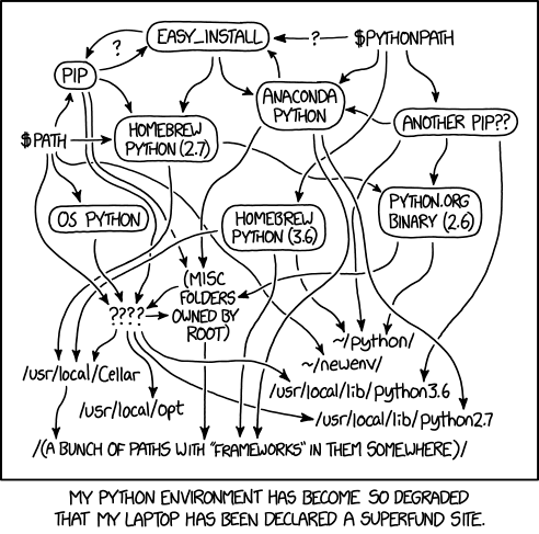
From XKCD (Creative Commons Attribution-NonCommercial 2.5 License)

Let us have a look at how we can create and manage virtual environments from the command line using venv and manage packages using pip.

Creating Virtual Environments Using venv

Creating a virtual environment with venv is done by executing the following command:

$ python3 -m venv /path/to/new/virtual/environment

where /path/to/new/virtual/environment is a path to a directory where you want to place it - conventionally within your software project so they are co-located. This will create the target directory for the virtual environment (and any parent directories that don’t exist already).

For our project let’s create a virtual environment called “venv”. First, ensure you are within the project root directory, then:

$ python3 -m venv venv

If you list the contents of the newly created directory “venv”, on a Mac or Linux system (slightly different on Windows as explained below) you should see something like:

$ ls -l venv

total 8
drwxr-xr-x  12 alex  staff  384  5 Oct 11:47 bin
drwxr-xr-x   2 alex  staff   64  5 Oct 11:47 include
drwxr-xr-x   3 alex  staff   96  5 Oct 11:47 lib
-rw-r--r--   1 alex  staff   90  5 Oct 11:47 pyvenv.cfg

So, running the python3 -m venv venv command created the target directory called “venv” containing:

• pyvenv.cfg configuration file with a home key pointing to the Python installation from which the command was run,
• bin subdirectory (called Scripts on Windows) containing a symlink of the Python interpreter binary used to create the environment and the standard Python library,
• lib/pythonX.Y/site-packages subdirectory (called Lib\site-packages on Windows) to contain its own independent set of installed Python packages isolated from other projects,
• various other configuration and supporting files and subdirectories.

Naming Virtual Environments

What is a good name to use for a virtual environment? Using “venv” or “.venv” as the name for an environment and storing it within the project’s directory seems to be the recommended way - this way when you come across such a subdirectory within a software project, by convention you know it contains its virtual environment details. A slight downside is that all different virtual environments on your machine then use the same name and the current one is determined by the context of the path you are currently located in. A (non-conventional) alternative is to use your project name for the name of the virtual environment, with the downside that there is nothing to indicate that such a directory contains a virtual environment. In our case, we have settled to use the name “venv” instead of “.venv” since it is not a hidden directory and we want it to be displayed by the command line when listing directory contents (the “.” in its name that would, by convention, make it hidden). In the future, you will decide what naming convention works best for you. Here are some references for each of the naming conventions:

• The Hitchhiker’s Guide to Python notes that “venv” is the general convention used globally
• The Python Documentation indicates that “.venv” is common
• “venv” vs “.venv” discussion

Once you’ve created a virtual environment, you will need to activate it.

On Mac or Linux, it is done as:

$ source venv/bin/activate
(venv) $

On Windows, recall that we have Scripts directory instead of bin and activating a virtual environment is done as:

$ source venv/Scripts/activate
(venv) $

Activating the virtual environment will change your command line’s prompt to show what virtual environment you are currently using (indicated by its name in round brackets at the start of the prompt), and modify the environment so that running Python will get you the particular version of Python configured in your virtual environment.

You can verify you are using your virtual environment’s version of Python by checking the path using the command which:

(venv) $ which python3

/home/alex/InterPython_Workshop_Example/venv/bin/python3

When you’re done working on your project, you can exit the environment with:

(venv) $ deactivate

If you’ve just done the deactivate, ensure you reactivate the environment ready for the next part:

$ source venv/bin/activate
(venv) $

Python Within A Virtual Environment

Within a virtual environment, commands python and pip will refer to the version of Python you created the environment with. If you create a virtual environment with python3 -m venv venv, python will refer to python3 and pip will refer to pip3.

On some machines with Python 2 installed, python command may refer to the copy of Python 2 installed outside of the virtual environment instead, which can cause confusion. You can always check which version of Python you are using in your virtual environment with the command which python to be absolutely sure. We continue using python3 and pip3 in this material to avoid confusion for those users, but commands python and pip may work for you as expected.

Note that, since our software project is being tracked by Git, the newly created virtual environment will show up in version control - since venv directories can get quite heavy, you’ll want to add them to the .gitignore file:

# Virtual environments
venv/
.venv/

Installing External Packages Using pip

We noticed earlier that our code depends on two external packages/libraries - pandas and matplotlib. In order for the code to run on your machine, you need to install these two dependencies into your virtual environment.

To install the latest version of a package with pip you use pip’s install command and specify the package’s name, e.g.:

(venv) $ pip3 install pandas
(venv) $ pip3 install matplotlib

or like this to install multiple packages at once for short:

(venv) $ pip3 install pandas matplotlib

How About python3 -m pip install?

Why are we not using pip as an argument to python3 command, in the same way we did with venv (i.e. python3 -m venv)? python3 -m pip install should be used according to the official Pip documentation; other official documentation still seems to have a mixture of usages. Core Python developer Brett Cannon offers a more detailed explanation of edge cases when the two options may produce different results and recommends python3 -m pip install. We kept the old-style command (pip3 install) as it seems more prevalent among developers at the moment - but it may be a convention that will soon change and certainly something you should consider.

If you run the pip3 install command on a package that is already installed, pip will notice this and do nothing.

To install a specific version of a Python package give the package name followed by == and the version number, e.g. pip3 install pandas==2.1.2.

To specify a minimum version of a Python package, you can do pip3 install pandas>=2.1.0.

To upgrade a package to the latest version, e.g. pip3 install --upgrade pandas.

To display information about a particular installed package do:

(venv) $ pip3 show pandas

Name: pandas
Version: 2.1.4
Summary: Powerful data structures for data analysis, time series, and statistics
Home-page: https://pandas.pydata.org
Author: 
Author-email: The Pandas Development Team <pandas-dev@python.org>
License: BSD 3-Clause License
...
Requires: numpy, python-dateutil, pytz, tzdata
Required-by: 

To list all packages installed with pip (in your current virtual environment):

(venv) $ pip3 list

Package         Version
--------------- -------
contourpy       1.2.0
cycler          0.12.1
fonttools       4.47.2
kiwisolver      1.4.5
matplotlib      3.8.2
numpy           1.26.3
packaging       23.2
pandas          2.1.4
pillow          10.2.0
pip             23.3.2
pyparsing       3.1.1
python-dateutil 2.8.2
pytz            2023.3.post1
setuptools      65.5.0
six             1.16.0
tzdata          2023.4

To uninstall a package installed in the virtual environment do: pip3 uninstall package-name. You can also supply a list of packages to uninstall at the same time.

Exporting/Importing Virtual Environments Using pip

You are collaborating on a project with a team so, naturally, you will want to share your environment with your collaborators so they can easily ‘clone’ your software project with all of its dependencies and everyone can replicate equivalent virtual environments on their machines. pip has a handy way of exporting, saving and sharing virtual environments.

To export your active environment - use pip3 freeze command to produce a list of packages installed in the virtual environment. A common convention is to put this list in a requirements.txt file:

(venv) $ pip3 freeze > requirements.txt
(venv) $ cat requirements.txt

contourpy==1.2.0
cycler==0.12.1
fonttools==4.47.2
kiwisolver==1.4.5
matplotlib==3.8.2
numpy==1.26.3
packaging==23.2
pandas==2.1.4
pillow==10.2.0
pyparsing==3.1.1
python-dateutil==2.8.2
pytz==2023.3.post1
six==1.16.0
tzdata==2023.4

The first of the above commands will create a requirements.txt file in your current directory. Yours may look a little different, depending on the version of the packages you have installed, as well as any differences in the packages that they themselves use.

The requirements.txt file can then be committed to a version control system (we will see how to do this using Git in one of the following episodes) and get shipped as part of your software and shared with collaborators and/or users. They can then replicate your environment and install all the necessary packages from the project root as follows:

(venv) $ pip3 install -r requirements.txt

As your project grows - you may need to update your environment for a variety of reasons. For example, one of your project’s dependencies has just released a new version (dependency version number update), you need an additional package for data analysis (adding a new dependency) or you have found a better package and no longer need the older package (adding a new and removing an old dependency). What you need to do in this case (apart from installing the new and removing the packages that are no longer needed from your virtual environment) is update the contents of the requirements.txt file accordingly by re-issuing pip freeze command and propagate the updated requirements.txt file to your collaborators via your code sharing platform (e.g. GitHub).

Keep in mind though that pip freeze won’t work properly if you’re using conda instead of venv - in fact, if you run pip3 freeze > requirements.txt from under conda environment, the result won’t be usable by pip itself, since it will produce the addresses of the local builds instead of package versions.

absl-py @ file:///croot/absl-py_1714140470852/work
aiohappyeyeballs @ file:///croot/aiohappyeyeballs_1734469393482/work
aiohttp @ file:///croot/aiohttp_1734687138658/work
...

What you want to use instead is pip list --format=freeze > requirements.txt, which will produce the output in pip-readable format.

Official Documentation

For a full list of options and commands, consult the official venv documentation and the Installing Python Modules with pip guide. Also check out the guide “Installing packages using pip and virtual environments”.

Installing Jupyter Lab

Jupyter Lab itself comes as a Python package. Therefore, we have to install it in the environment as well. Another package that we will need for our project is astropy, which provides a lot of functions, useful for writing astronomical software and data processing.

(venv) $ pip3 install astropy
(venv) $ pip3 install jupyterlab

Do not forget to update the requirements.txt file after the installation is finished. If you run pip freeze, you will see that Jupyter Lab installed a lot of dependencies libraries, so the list of requirements is now much larger.

Key Points

• Virtual environments keep Python versions and dependencies required by different projects separate.

• A virtual environment is itself a directory structure.

• Use venv to create and manage Python virtual environments.

• Use pip to install and manage Python external (third-party) libraries.

• pip allows you to declare all dependencies for a project in a separate file (by convention called requirements.txt) which can be shared with collaborators/users and used to replicate a virtual environment.

• Use pip3 freeze > requirements.txt to take snapshot of your project’s dependencies.

• Use pip3 install -r requirements.txt to replicate someone else’s virtual environment on your machine from the requirements.txt file.

Integrated Software Development Environments

Overview

Teaching: 10 min
Exercises: 5 min

Questions

• What are Integrated Development Environments (IDEs)?

• What are the advantages of using IDEs for software development?

• How does Jupyter Lab interact with virtual environments?

Objectives

• Set up Jupyter Lab and its kernels

• Use Jupyter Lab to run a script

Introduction

As we have seen in the previous episode - even a simple software project is typically split into smaller functional units and modules, which are kept in separate files and subdirectories. As your code starts to grow and becomes more complex, it will involve many different files and various external libraries. You will need an application to help you manage all the complexities of, and provide you with some useful (visual) facilities for, the software development process. Such clever and useful graphical software development applications are called Integrated Development Environments (IDEs).

Integrated Development Environments

An IDE normally consists of at least a source code editor, build automation tools and a debugger. The boundaries between modern IDEs and other aspects of the broader software development process are often blurred. Nowadays IDEs also offer version control support, tools to construct graphical user interfaces (GUI) and web browser integration for web app development, source code inspection for dependencies and many other useful functionalities. The following is a list of the most commonly seen IDE features:

• syntax highlighting - to show the language constructs, keywords and the syntax errors with visually distinct colours and font effects
• code completion - to speed up programming by offering a set of possible (syntactically correct) code options
• code search - finding package, class, function and variable declarations, their usages and referencing
• version control support - to interact with source code repositories
• debugging - for setting breakpoints in the code editor, step-by-step execution of code and inspection of variables

IDEs are extremely useful and modern software development would be very hard without them. There are a number of IDEs available for Python development; a good overview is available from the Python Project Wiki. In addition to IDEs, there are also a number of code editors that have Python support. Code editors can be as simple as a text editor with syntax highlighting and code formatting capabilities (e.g., GNU EMACS, Vi/Vim). Most good code editors can also execute code and control a debugger, and some can also interact with a version control system. Compared to an IDE, a good dedicated code editor is usually smaller and quicker, but often less feature-rich. You will have to decide which one is the best for you - in this course, we will use Jupyter Lab - a free open-source web-based IDE familiar to most Python-coding astronomers.

Is Jupyter Lab an IDE?

For a long time, Jupyter Notebook was not considered as a full-fledged IDE. The main argument against considering Jupyter Notebooks an IDE was that it lacked a lot of functionality that is essential for the full cycle of software development. The most notable instrument that wasn’t present in Jupyter Notebook was the debugger.

However, modern versions of Jupyter Lab, an evolutionary development of Jupyter Notebook, come with the built-in debugger, as well as with all the rest of the basic IDE instruments. Formally, this makes Jupyter Lab a ‘real’ IDE. At the same time, Jupyter Lab and classic IDEs (such as PyCharm or Spyder) impose distinctly different coding routines. Jupyter Lab (as Jupyter Notebook before) assumes an interactive cell-by-cell development and execution of the code, which is well-suited for data exploration and analysis and for small-scale software development. At the same time, for larger projects that do not require executing small parts of the code separately, ‘classic’ IDEs are more suitable.

Using Jupyter Lab

Let’s open our project in Jupyter Lab now and familiarise ourselves with some commonly used features.

Jupyter Lab interface

To launch Jupyter Lab, activate the venv environment created in the previous episode and type in the terminal:

 (venv) $ jupyter lab

The output will look similar to this:

 To access the server, open this file in a browser:
        file:///home/alex/.local/share/jupyter/runtime/jpserver-2946113-open.html
    Or copy and paste one of these URLs:
        http://localhost:8888/lab?token=e2aff7125e9917868a16b8b627f73995eb83effbcafeee05
        http://127.0.0.1:8888/lab?token=e2aff7125e9917868a16b8b627f73995eb83effbcafeee05

Now you can click on one of the URLs below and Jupyter Lab will open in your browser.

Jupyter Lab starting interface

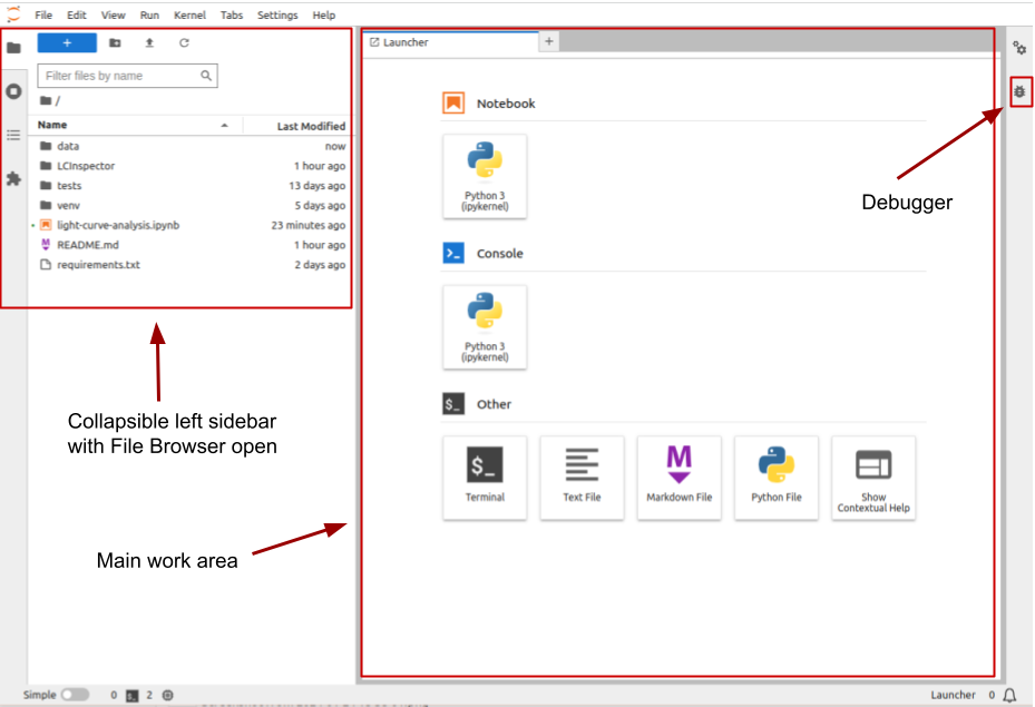
The Jupyter Lab interface includes the following areas:

1. Menu bar, from which you can access most common Jupyter Lab functions;
2. A collapsible left sidebar, in which four tabs are present:
   • File Manager. From here you can manage the files and directories in your repository folder.
   • Running terminal and kernels. Here you can find the list of running Jupyter Notebook kernels and console sessions.
   • Table of contents. Here Jupyter Lab will automatically generate a table of contents of your notebooks (using headers and other markdown cells) and Python files (using function and class definitions).
   • Extension Manager. In this section, it is possible to install extensions that expand Jupyter Lab functionality, for example, allowing integration with Git, adding CSS formatting, and so on.
3. The main work area. When you just opened Jupyter Lab, you can see several options for starting your work, such as creating a new Notebook, opening a new Python console session, or creating a new text or Python file. The list of these options will vary depending on which kernels and programming languages you have installed. When you open a Notebook or a file, it will appear in a separate tab in this area.
4. In the right collapsible sidebar you can access the notebooks’ Properties Manager and Debugger, which can be used for inspecting the variables and managing Breakpoints.

Making Jupyter Lab show hidden files

By default, Jupyter Lab file manager does not show hidden files. If you prefer to change that, you need to enable a corresponding option in Jupyter Lab configuration file. In the terminal run:

$ jupyter --paths

config:
    /home/alex/.jupyter
    ...
data:
    /home/alex/.local/share/jupyter
    ...

This command lists the folders in which Jupyter will look for configuration files, ordered by precedence. In all likelyhood, you already have a config file called jupyter_server_config.py in the upmost folder:

$ ls -l /home/alex/.jupyter

total 84
-rw-rw-r-- 1 alex alex 69714 Jul  1 12:38 jupyter_server_config.py
drwxrwxr-x 4 alex alex  4096 Feb  4 14:28 lab
...

If not, you can generate it by typing:

$ jupyter server --generate-config

Next, open it with any text editor, for example:

$ gedit /home/alex/.jupyter/jupyter_server_config.py 

and find c.ContentsManager.allow_hidden parameter. By default it is commented out and set to False, so you need to uncomment it and change its value to True, and then save the file.

After that go to the Jupyter Lab window and choose View > Show hidden files, and hidden files will be available through the Jupyter Lab file browser. It is handy when you need to edit some hidden configuration files or keep track on temporal files created by your code, and if you don’t need it for some particular project, you can always switch it off by unchecking View > Show hidden files.

Opening a Software Project

In the left sidebar, open the File Browser and look through the files present here. You can inspect the requirements.txt file, where we saved the list of packages installed in our virtual environment, and README.md, containing some basic information about the project. Later we will add more information to this file. For now, double click on the light-curve-analysis.ipynb.

In the opened tab we can see a number of cells. Some of them contain Python code, while others display formatted text (‘Markdown’). You can change the type of the cell in the drop-down menu in the instrumental panel on the top of the tab. You can execute cells one by one by pressing Shift+Enter, or run them all by choosing Run > Run All in the main menu or by pressing a corresponding button in the tab instrumental panel. Code cells produce outputs, which may contain text, tables and static or interactive plots.

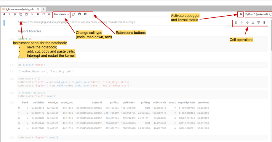
Interface elements of a notebook tab

By default the notebooks are opened in tabs that take the full screen, however, you can align them vertially or horizontally by dragging them in the preferred place. You can also place an output of any cell into a separate tab. For this, make a right-click on the output content and choose Create New View for Cell Output. You can open multiple tabs for the cell outputs and reorder them in the same way as the notebook tabs.

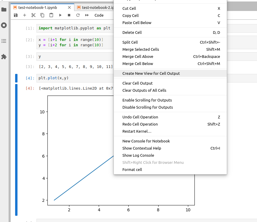
Creating cell output view

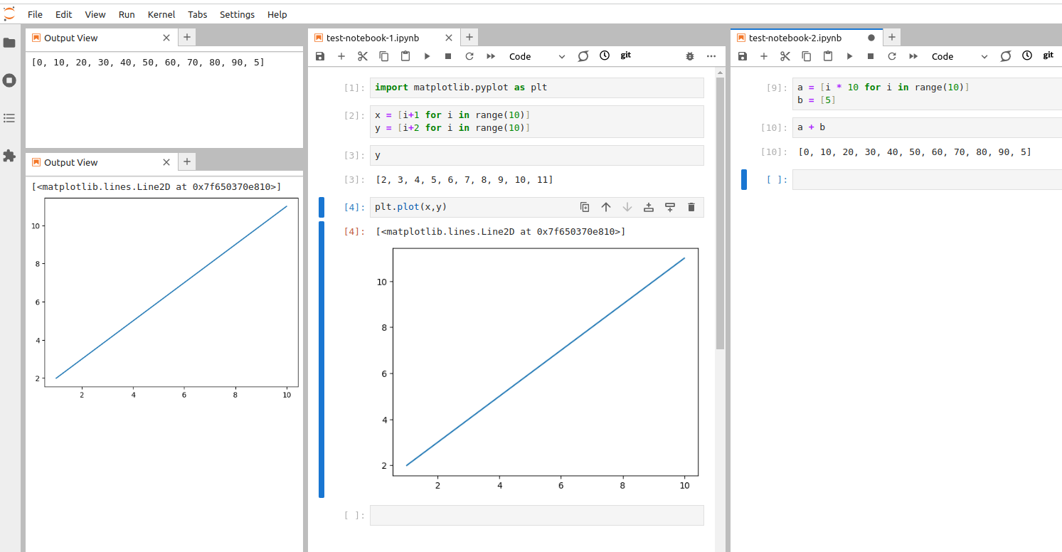
You can order the notebook tabs and cell output views any way you like

The code in the notebook is displayed using different colours, following the rules set up for the syntax highlighting. Syntax highlighting is a feature that displays source code terms in different colours and fonts according to the syntax category the highlighted term belongs to. It also makes syntax errors visually distinct. Highlighting does not affect the meaning of the code itself - it’s intended only for humans to make reading code and finding errors easier. The code highlighting color scheme depends on the programming language (or, to be more precise, on the kernel which is currently connected to your Notebook), and in the Text Editor, you can pick the language yourself in View > Text Editor Syntax Highlighting menu. By default it is inferred from the file extension, e.g. Python for .py files.

Code Completion & Documentation References

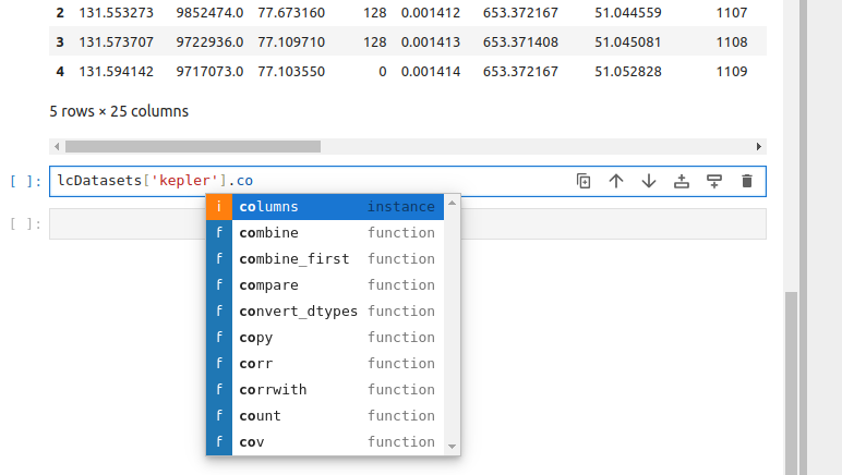
Context-aware code completion suggestions (`Tab`)

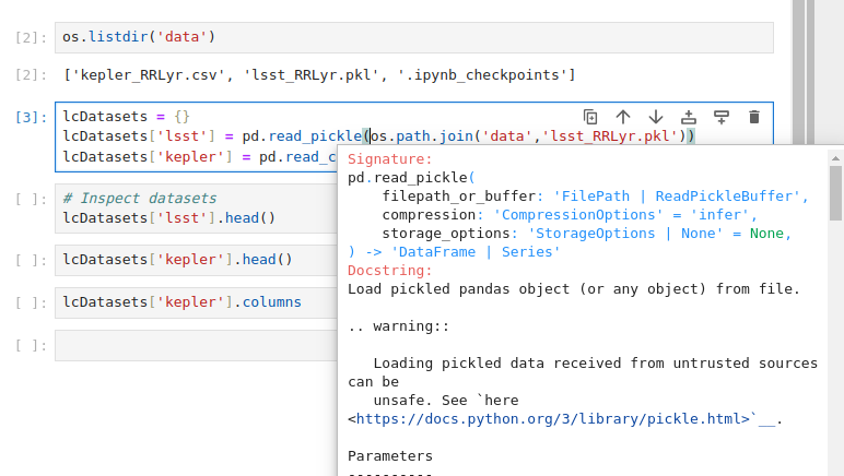
Contextual help in a pop-up window (`Shift+Tab`)

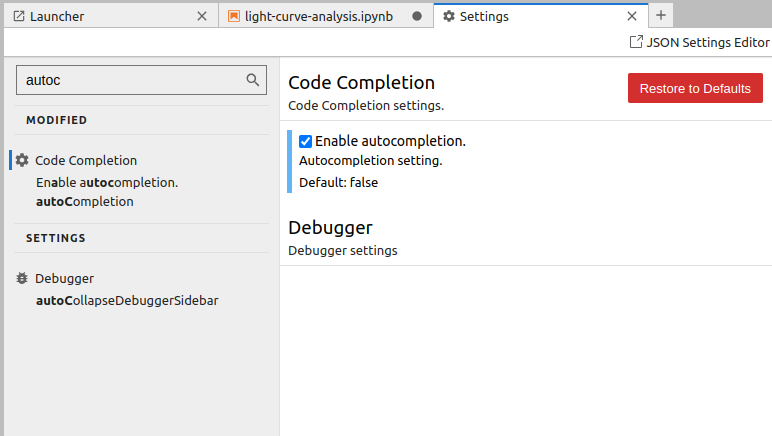
Setting up auto-completion

When you are typing code, you can use completion suggestions and contextual help tools, included in Jupyter Lab. You can use three hotkey combinations for using these tools:

1. When you start typing a command, you can press Tab, and Jupyter Lab will offer you options of code that can follow.
2. You also can type Shift+Tab to open contextual help in a pop-up window.
3. Another option is to use Ctrl+I for opening contextual help in the right sidebar.
4. Finally, you can enable code auto-completion. For this, go to ‘Settings > Settings Editor’ and start typing ‘auto-completion’ in the Search box. Then select the ‘Enable autocompletion’ checkbox.

Using context-aware code completion features speeds up the process of coding, and reduces typos and other common mistakes. Using contextual help also improves the quality of the code, as well as simplifies the process for the programmer.

How does contextual help work?

Contextual help relies on the docstrings, written in the library’s source files by the developers. If you look at code definitions of well-maintained libraries, such as Pandas or Numpy, you will see that the docstrings are very detailed: they contain input parameters, outputs, algorithm descriptions, and even examples of usage. Later we will talk about how to write good docstrings, but here you can see why they are so essential.

Try completion, auto-completion, and contextual help functions

Execute already existing cells of the notebook. There are several ways to do this:

1. You can go through the cells, clicking Shift+Enter on each of them.
2. You can use Run > Run all cells menu.
3. You can use Restart the kernel and run all cells button on the tool panel on the top of your notebook tab. Be aware that when you restart the kernel, you lose all the data from already executed code, e.g. all the variables will be deleted.

After that, inspect contextual help of several functions, e.g. pd.read_pickle, np.array, and os.path.join. Pay attention to which information is included in the contextual help and in which format. Next, get the list of the columns in one of the opened datasets, using completion at every step.

Solution

To get the list of the columns you can use the following code: LcDatasets['kepler'].columns. By pressing Tab once you started typing ‘LcDatasets’, ‘kepler’ and ‘columns’, you will get suggestions for the available options of the following code.

After that, enable auto-completion and get the list of the columns of the second dataset. Depending on what is more convenient for you, you can leave auto-completion function turned on, or turn it off.

Code Search

Jupyter Lab offers you the possibility to search and replace text within the file, using case matching and regular expressions. You can perform the search within the whole document or only in a single cell, with or without cell outputs (the results of execution of the code within the cell). To access the search tool, use Ctrl+F key combination, or Edit > Find in the main menu.

Searching across multiple notebooks

Jupyter Lab built-in search does not allow searching strings across multiple files. However, such functionality is available with jupyterlab-search-replace extension.

Key Points

• An IDE is an application that provides a comprehensive set of facilities for software development, including syntax highlighting, code search and completion, version control, testing and debugging.

• Jupyter Lab launches within the pre-existing virtual environment

• We can run terminal commands within Jupyter Lab

Best practices for Jupyter

Overview

Teaching: 10 min
Exercises: 5 min

Questions

• How to avoid chaos when writing code in Notebooks?

• What is the workflow when using Jupyter Lab for software development?

Objectives

• Follow best practice to ensure that your Notebook is well-organized and reusable.

Pros and Cons of Interactivity

Jupyter notebooks are very convenient since they allow executing pieces of code in an arbitrary order, giving the developer a high level of interactivity. The other side of the coin is that notebooks enable the development of the code without a clear structure, and that the result of the executed code differs depending on which cells were executed prior to that. Taking care of keeping the code in order falls on the developer’s shoulders even more than when a classic IDE is used.

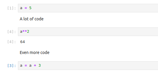
Inattention to cell execution order can mess your data

As a result, Jupyter Lab is not recommended for large-scale software development, and even for smaller projects the final code should always be extracted into executable ‘.py’ files and converted into Python package. At the same time, notebooks are well-suited for data inverstigation, visualization and presentations, and it is the best when .ipynb files contain only the code related to those tasks. Even then, without following certain best practices, notebooks have poor reproducibility.

Jupyter Lab best practices

Fortunately, Jupyter Lab provides us with a number of tools that allow us to keep the notebook files clean, and the developed code reliable. Let’s consider the most important rules of keeping your notebooks in a good condition:

1. Set the objective. Define the objective of the notebook from the start and write it on the top of the notebook. Pay attention to how you phrase the objective: it should explain what is done in this notebook and be specific. E.g. instead of generic ‘Some code for analysing the data’ it is better to write ‘Inspect, clean from NaNs and visualize on a histogram LSST RR Lyrae light curves dataset’.
2. One notebook - one task. One notebook should correspond to only one task or stage of your investigation. E.g. it is better to separate data preprocessing and visualization, or analysis of the spectra and analysis of the light curves. Do not stray from this objective; you definitely will get new ideas while working on your analysis, but if they are outside of the scope of this particular notebook, they should be extracted to a new file. There are two possible exceptions to this rule: if your notebook is really small (e.g. you just need to make a couple of plots), or if it’s a demonstration or presentation notebook.
3. Structure first.Think about the structure of the notebook before you start working, and write the headers of the sections in advance. For most astronomical projects, you will need at least four sections: imports, loading the data, pre-processing the data and analysis itself. Remember, that you can create subsections using secondary headers! It is also a good idea to put variables, that later will be used across the code (e.g. sizes of samples, time ranges for period search, magnitude limits) into a separate section before the analysis, and create temporary sections for classes and functions (which ultimately should be extracted into .py files).
4. Utilize Markdown cells for detailed explanations of what is done in the following code cells. Markdown cells allow you to use headers, common types of text formatting, such as bold, italics and strikethrough formatting, create lists, separators and tables, insert latex equations and use HTML formatting and so on. Here is a cheat sheet for the common types of formatting. To convert the cell into Markdown, you can press Esc and then M, or by using the drop-down menu in the instrumental panel at the top of the notebook tab.

5. Keep it short. Keep your notebooks short. There is no hard rule, but constraining a notebook to a hundred of cells is a good idea. If your notebook is longer than that, make sure that you follow the rule of ‘One notebook - one task’.

   Jupyter Lab Table of Contents

   The benefit of using multi-level headers for sections and subsections is that Jupyter Lab uses them for creating the Table of Contents, which can be accesses from the collapsible left side-bar. With this panel, you can quickly evaluate the structure of your notebook, go to any subsection or execute all the cells under the selected header.

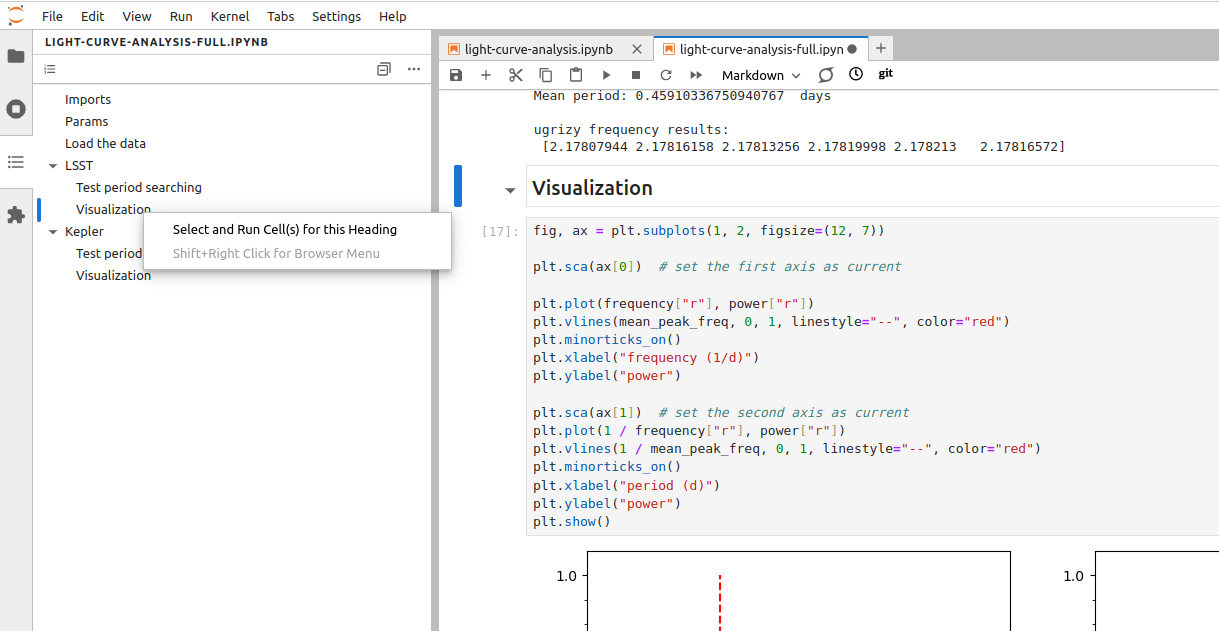
   Using the Table of Contents to execute cells in a selected section

   Fix the structure of the ‘light-curve-analysis.ipynb’ notebook

   Go through the best practices listed above one by one and improve the structure of the light-curve-analysis.ipynb notebook.

   Solution

   Let’s go through the recommendations one by one.

   1. Set the objective. Right now the objective of the notebook is phrased in a generic way. We can rephrase it into, e.g. ‘Inspect the sizes and visualize light curves from the LSST and Kepler RR Lyrae datasets.’
   2. One notebook - one task. Since for now our notebook is small, we can leave it as it is. However, potentially we could have put visualization into a separate notebook.
   3. Structure first. Currently the structure of the notebook is not well-defined. Add headers for the sections dedicated to the inspection of the datasets and visialization of a light curve, put all imports into the corresponding section and move the variables that we are likely to use in different sections to the ‘Params’ section (in our case it can be plot_filter_labels, plot_filter_colors and plot_filter_symbols).
   4. Keep it short. Since our notebook has less than a hundred cells, for now we don’t have this problem.
   5. Utilize Markdown cells. Give a brief description for each section (you can put it in the same cell as the headers). Use some formatting, e.g. in the ‘Dataset inspection’ section create a table listing the number of objects in current versions of each of the datasets.

   What about the code that has to be executed only once, and then skipped?

   Let’s say you have some code that has to be executed only once, and in the next executions of the notebook it has to be skipped. Such situations often arise during data pre-processing, when some data has to be downloaded or cleaned from NaNs only once, and in the subsequent executions of the notebook loaded from the saved copy. Taking these pieces of code into a separate notebook is not always convenient, and using comments to make this code inactive makes your notebook hard to understand in the future. A good way to handle such situations is to use boolean flags to indicate which steps have to be executed, and which should be skipped. By storing these flags in the ‘Parameters’ section you can quickly see the current state of your work, and turn on and off different steps of the data processing as needed.

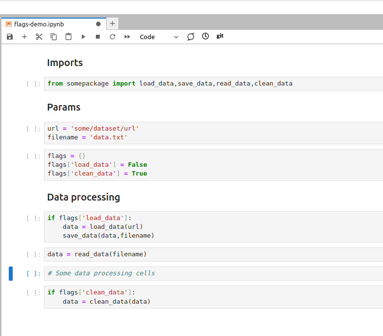
   Using boolean flags to indicate parts of the code that has to be skipped

6. Keep an eye on performance. If your notebook contains pieces of code that are computationally expensive, work on a small representative sample of the data instead. When the code is ready, convert it into an executable .py file and launch it from terminal. It will help you to avoid situations when the result of a long computation is lost due to the IDE crash, and also it will make it possible to launch your analysis on the machines where Jupyter Lab is not available, e.g. on a remote server.
7. Reuse your code wisely. The code that you use more than once has to be turned into functions. This recommendation is applicable in all situations, not only when you use notebooks.
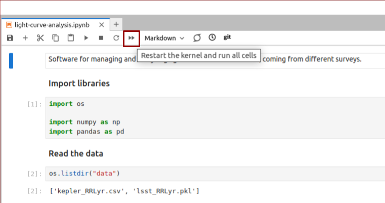
8. Package your code. It is convenient to use Jupyter Lab for developing your code, however, once it is ready and tested, you should extract your classes and functions into .py files and then turn it into a Python package. This allows you to use this code again across multiple notebooks, in other IDEs or from command line. In the next few days we will talk more about how to package your code.
9. Use ‘Restart and Run All’ often. Executing cells out of order is one of the main source of errors when developing code in Jupyter Lab. For this reason, make a habit of regularly using the ‘Restart and Run All’ button, that will restart your kernel, delete all stored variables and execute all cells in the top-down order. Always do it before saving the notebook and pushing it into a Git repository. This habit greatly improves the reproducibility of your notebooks.

'Restart and Run All' button helps you to ensure that your notebook is executed in the right order

Shouldn’t We Clear Outputs of All Cells Before Pushing the Notebook into a Repo?

There is an old recommendation to always use Restart Kernel and Clear Outputs of All Cells before committing the notebook into a Git repository. This recommendation comes from the fact that native Git tools for comparing different versions of the files (git diff) do not handle .ipynb files well. Plots in the outputs are especially inconvenient, since they will show up as human-unreadable strings (which is what images are when you try to open them via text editor). However, git diff in general isn’t suitable for investigating changes in any files that are not, in essence, plain text. More so, clearing the outputs of the notebooks after you finished your work makes it impossible to e.g. use the notebook for a spontaneous presentation or demonstration of the results. The solution to this problem is to use the suitable instruments. Jupyter Lab has several extensions that allow to compare different versions of the notebooks, such as nbdime and jupyterlab-git. More so, currently GitHub provides us with a possibility to use so called ‘Rich Jupyter Notebook Diffs’ when an updated notebook is pushed in your repository. You can enable this function by clicking on your avatar in the top right corner and then selecting Feature Preview > Rich Jupyter Notebook Diffs.

Jupyter Notebook, Rubin Science Platform and Google Colab

While RSP and Google Colab have Jupyter Notebook installed and not Jupyter Lab, all of the best practices above are still applicable on these platworms, with the only exception that you will have to create the Table of Contents manually.

Additional exercise

Open one of your recent notebooks and apply the best practices listed above to improve its structure. Do you need to reorder your code a lot? Is there some code that can be extracted into .py files?

Key Points

• The interactivity of Notebooks, while convenient, enables chaotic style of software development.

• We must follow best practices for Jupyter Lab to avoid chaos in the Notebooks.

Jupyter Magics and Resource Profiling

Overview

Teaching: 10 min
Exercises: 10 min

Questions

• What is software profiling?

• What tools can we use to measure time and computational resources required by our software?

Objectives

• Use Jupyter magics and SnakeViz to profile time and computational resources.

What is Software Profiling?

We may have a software that is doing everything that we want it to do, with its codebase well-written and perfectly comprehensible, but this does not yet guarantee that this software will be applicable to the real-world problems. For example, its interface can be so convoluted that the user can’t figure out how to access the feature of interest. Other common issue is when the software has such high computational complexity that it can be used only on small datasets, or on computer clusters with hundreds of GB of memory.

The process of estimating how much time the execution of the software will take and how much memory or other resources it will need is called profiling. Profiling is a form of dynamic program analysis, meaning that it requires launching the software and measuring its performance and logging its activity as it runs. One of the main purposes of profiling is to identify bottlenecks, inefficient operations, or high-latency components of the program, so that these parts could be optimized to run faster or to use less resources. It is worth noting that for many problems there is a space-time tradeoff, which essentially means that by optimizing the program in respect to the execution time we make it less memory-efficient, and vice versa.

How necessary profiling is for academic software development? Well, it is ok to skip profiling when working on small projects that can be easily executed on your PC or within a Google Colab notebook. However, as your projects get larger, the execution of your code may start taking days and weeks, or it may start crashing due to the lack of RAM or CPU power. Another example when the efficiency is crucial is executing your code at astronomical data access portals, such as Rubin Science Platform or Astro Data Lab. These platforms provide an opportunity to work with large astronomical datasets without downloading them to your machine, however, the CPU and memory allocated to each user are limited. Code profiling helps us to determine which implementation is more efficient and to make our code scalable. And if you are developing software that will be used by someone else, it also makes the users happier (and in some cases ensures that the software will be used at all).

In this introduction to profiling we mostly concentrate on time profiling, with some notes on memory profiling. We start with the Jupyter built-in tool, Jupyter Magics.

What Are Jupyter Magics?

Jupyter Magics are special commands in Jupyter Notebooks/Lab that extend functionality by providing shortcuts for tasks like timing, debugging, profiling, or interacting with the system, e.g. executing terminal commands from withing the notebook. They come in two forms:

• Line Magics: Prefixed with %, they operate on a single line of code.
• Cell Magics: Prefixed with %%, they apply to the entire cell.

Why Magics aren’t really part of the Jupyter

To be specific, Magic commands are part of the Python kernels that are used by the Jupyter Notebook or Lab. The kernels are separate processes, language-specific computational engines that are executing the commands you gave it with the code. The kernel with which your notebooks is launched is separate from the frontend processes that handle, for example, the tasks of adding or removing cells, or even rendering the characters when you type them during the execution of the previous cell. Think on how different it is from when you launch some commands in your PC terminal: there, you cannot type the next commands until the previous one finish executing. The separation of the Jupyter frontend from the kernel is what allows to avoid this behavior.

By default, Jupyter uses ipykernel, and Magic commands are a part of it. However, many different kernels for Jupyter exist, including some developed for other languages, such as R or Julia. Whether Magic commands are available for these kernels depends on their implementation.

If you want to know more how kernels work, here is a generic overview with some practical examples.

Here is a short list of the most useful magics:

• %magic: prints information about magics system
• %lsmagic: lists all magic commands in a convenient form
• %quickref: another helper function that shows references for the magic commands
• %time, %timeit and %%timeit: measure the execution time of the code.
• %cd, %ls, %pwd and other console commands: executes terminal commands
• %run: executes another ‘.ipynb’ or ‘.py’ file from within the current notebook
• %who: lists the defined variables. It is possible to list only variables of a certain type, e.g. %who string.

There are plenty Magics cheatsheets online, however, the easiest way to look up what kinds of comands are there is to use Magics itself:

• %lsmagic - prints a list of all Magics available;
• %quickref - prints a reference card on the available Magic commands.

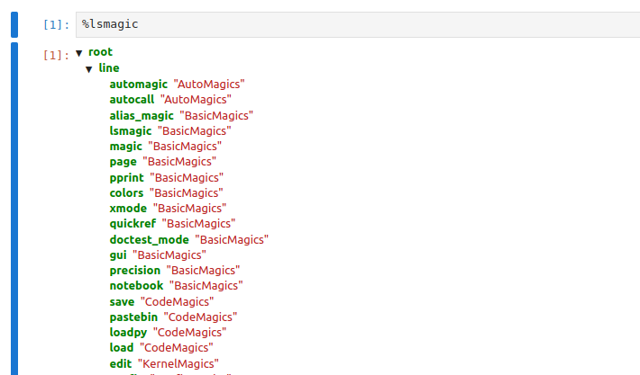
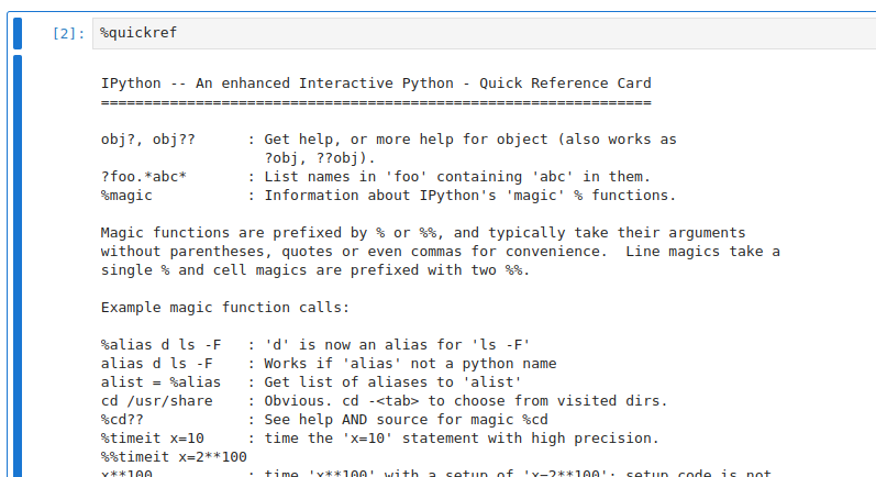
Try out different magics

Try several different magic commands, such as %lsmagic, %pwd and %who. Use %who command to get the list of dict variables (pay attention, that if you use %who command without specifying the type of the variable, it will also include the packages that you imported in the notebook).

Apart from the built-in magics, there are many more that you can install additionally. It is also possible to develop your own magic commands.

Installing packages from Jupyter notebook interface or Jupyter console session

Since magics allow us to execute terminal commands, there is a way to install Python packages right from the Jupyter interface. We can run %pip3 install astropy right in a Jupyter cell. This is a standard way of installing packages in cloud Jupyter Notebook services, such as Google Colab or the Notebook aspect of Rubin Science Platform. Pay attention, though, that another common way of doing this, using ! instead of % before the installation command, is in general not safe and can lead to the dependencies issues due to the particularities of how OS and Jupyter kernels interact. You can still see it often, since magic command for pip appeared only in the later versions of IPython.

Time Profiling with Magics

For time profiling, the most useful Magics are:

• %time: Measures execution time of a single line.
• %%time: Measures execution time of an entire cell.
• %timeit: Repeats timing of a line for reliable results.
• %%timeit: Repeats timing of a cell for average results.

Let’s use this function to profile some code. As an example we’ll use a code that calculates the first thousand of partial sums of series of natural numbers and saves it into a list.

First, we need to create a new branch:

$ git checkout develop
$ git checkout -b profiling

Then let’s write one possible implementation of the code for the problem above:

%%time
# Example: Timing a block of code
result = []
for i in range(1000):
    result.append(sum(range(i)))

This code creates an empty list result, and then launches a for loop in which for each i in the range from 0 to 1000 a sum of all numbers from 0 to i is calculated and appended to the list. This code produces the following output:

CPU times: user 10.4 ms, sys: 0 ns, total: 10.4 ms
Wall time: 10.2 ms

As you can notice, there are several measurements taken:

• Wall Time: Total elapsed time from start to end of a task, including waiting time for I/O operations or other processes.
• CPU Time: The time the CPU spends executing the code, further divided into User Time (time spent executing user code) and System Time (time spent on system-level operations, such as I/O or memory management).
• In general, there is also Overhead, which is the additional time introduced by profiling tools themselves, which may slightly skew results.

The double %% symbol means that %%time is applied to entire cell. Pay attention that if you use %time instead, the result will be very different:

CPU times: user 2 μs, sys: 0 ns, total: 2 μs
Wall time: 4.05 μs

2 microseconds (since it’s μs and not ms) instead of ten milliseconds. These microseconds is the measurement of an execution time of an empty line, since %time command does not care about the code in the following lines.

If you launch the code above several times, you’ll notice that the measured time can differ quite a lot. Depending on the specifics of the code and on the usage of system resources by other processes, the runtime of a code block may vary. As a side-remark, if you develop code running on a spacecraft, you want to avoid unpredictable runtime at all cost. To get a better measurement, %timeit and %%timeit runs the code seven times and produces mean and standard deviation of the execution time. This command also discards outlying measurements that are likely caused by temporary system slowdowns (e.g. caused by other software that is running on your PC).

%%timeit
# Example: Timing a block of code with 'timeit'
result = []
for i in range(1000):
    result.append(sum(range(i)))

4.43 ms ± 35.2 μs per loop (mean ± std. dev. of 7 runs, 100 loops each)

The 7 runs, 100 loops each tells us that the code was executed 7x100 times in total. While 7 runs is the set default value, the number of the loops is calculated automatically depending on how fast your code is, so that profiling didn’t take too much time. You can change the number of runs and loops using the flags -n and -r, for example, like this: %%timeit -n 4 -r 10 to run the code 4 times, with 10 loops in each run. Another useful flag is -o that allows you to store the result of the profiling in a variable:

%%timeit -n 4 -r 10 -o
# Example: Timing a block of code with saving the profiling result
result = []
for i in range(1000):
    result.append(sum(range(i)))

# In a new cell we save the content of the temporary
# variable '_' into a new variable 'measure'
measure = _
measure

<TimeitResult : 5.16 ms ± 1.56 ms per loop (mean ± std. dev. of 10 runs, 4 loops each)>

measure variable is a TimeitResult object that has some useful methods that allow us to see e.g. the value of the worst measurement and the measurements of all runs.

Memory Profiling with Magics

On machines with limited RAM, we could also consider profiling memory usage. For this we can install more magic commands, e.g. from Python Package Index

$ python -m pip install ipython-memory-magics

and load the external memory magic via

%load_ext memory_magics

Now we can analyze the memory usage in our cell

%%memory
# Example: Memory usage
result = []
for i in range(1000):
    result.append(sum(range(i)))

The output of this should look as follows:

RAM usage: cell: 35.62 KiB / 35.79 KiB

This reports current and peak memory usage of the code. Another useful option is to use %memory -n command in an empty cell, which will print how much RAM the whole current notebook is taking.

RAM usage: notebook: 158.61 MiB

Execution time with Magics

Use Magic commands to measure execution time for functions max_mag and plot_unfolded.

Solution

Either in a new section of the light-curve-analysis.ipynb notebook or in a new notebook we can import the max_mag function and use %time command:

from lcanalyzer.models import max_mag
...
%time lcmodels.max_mag(lc[lc_bands_masks[b]],mag_col=mag_col)

CPU times: user 1.94 ms, sys: 155 μs, total: 2.1 ms
Wall time: 1.9 ms
np.float64(18.418037351622612)

And we see that this command takes only a few microseconds to run. Pay attention that in order for this command to work, it should be in the same line as the code you are profiling. Otherwise, you need to use a cell Magic preceded by %%.

Next use %timeit on a plotting function:

%timeit views.plot_unfolded(lc[lc_bands_masks[b]],time_col=time_col,mag_col=mag_col,color=plot_filter_colors[b],marker=plot_filter_symbols[b])

347 ms ± 9.54 ms per loop (mean ± std. dev. of 7 runs, 1 loop each)

Wow, what happened? We got seven copies of the same plot! This is because %timeit repeats the execution and measures the average time. Plotting also takes noticeably longer time that a simple calculation of a maximum value.

A Few Words on Optimization

Let’s take our ‘partial sums of series’ problem and think on how we can optimize it to run faster. You may remember that Python has list comprehensions syntax that is sometimes recommended as a faster tool than for loops. We can rewrite the code above to use list comprehensions and use %%timeit magic to profile it.

%%timeit
# Implementation with list comprehension
result = [sum(range(i)) for i in range(1000)]

4.43 ms ± 71 μs per loop (mean ± std. dev. of 7 runs, 100 loops each)

Well… Actually, we got pretty much the same result. For this particular case, there is no computational gain in using list comprehension, although the code is cleaner and more readable this way. However, if we experiment with the maximum value of the range, we’ll start noticing the gain with the increase of this value. That said, for some problems list comprehensions may work even slower than for loops, which is why time profiling is something to do before you start optimization - it may turn out that the bottleneck is in a completely different part of the program than you thought. In order to optimise this specific piece of code, we would have to be smarter and use an equation instead of the bruteforce approach:

%%timeit
# Optimized implementation using mathematical formula for summation
result = [(i * (i - 1)) // 2 for i in range(1000)]

77.6 μs ± 812 ns per loop (mean ± std. dev. of 7 runs, 10,000 loops each)

Now the execution time is in dozens of microseconds, which is two orders better than before! That’s quite an improvement.

What If You Don’t Use Jupyter?

Of course, Jupyter Magics isn’t the only tool for time profiling. In fact, Python has built-in modules just for this, such as time and timeit, that can be used in any IDE.

import time
...
start_time = time.time()
max_mag = lcmodels.max_mag(lc[lc_bands_masks[b]],mag_col=mag_col)
print(f"Execution time: {time.time() - start_time:.5f} seconds")

Execution time: 0.00083 seconds

In this snippet of code, time.time() function records the current time in seconds since the epoch (typically January 1, 1970). This value is stored in the variable start_time before the code block is executed. After the code block, time.time() is called again to get the current time. The difference between the current time and start_time gives the total execution time. This elapsed time is formatted to five decimal places and printed. The time library is useful also in notebooks, when we want to get a detailed execution time log from the inside of a larger piece of code, e.g. a function.

To get a more reliable estimate, for the small snippets of code we can use timeit.repeat() method. It executes the timing multiple times and provides a list of results, making it easier to analyze performance under changing environments.

import timeit
results = timeit.repeat('sum([i**2 for i in range(1000)])', repeat=5, number=1000)
print("Timing Results:", results)
print("Best Execution Time:", min(results))

Timing Results: [0.17868508584797382, 0.16405000817030668, 0.16924912948161364, 0.1637995233759284, 0.16636504232883453]
Best Execution Time: 0.1637995233759284

The repeat and number parameters of this function work similarly to the number of runs and number of loops for the %%timeit. However, this method cannot be used conveniently for e.g. measuring execution time of functions. For this, we need a more advanced tool.

Additional reading on ‘time’ module and

Some additional sources to look into are:

• Python timeit Module: Detailed explanation of how to use the timeit module for benchmarking Python code.
• Python time Module: Overview of the time module, including functions like time(), sleep(), and more.
• Profiling in Python: A beginner-friendly introduction to time profiling methods in Python.

Resource profiling with offline profilers

Jupyter Magics, while extremely useful for small-scale profiling, aren’t a suitable tool for larger projects. Prioritizing development requires to understand multiple aspects of the code ‘under-the-hoods’:

• The frequency at which a function is called,
• The execution time for each function,
• The performance of different algorithms,
• Benchmarking pure python vs external C code,
• Identify bottlenecks and gauge how involved a change is compared to the development effort.

There are numerous tools for these inquiries. Here we will consider the cProfile and snakeviz modules.

cProfile is a built-in Python module that measures how many times each function was called from within the code that is being profiled and how much time the execution of each function took. cProfile is partially written in C, which makes it faster and reduces the overhead that is inevitably added by any profiler. If cProfile doesn’t work on your PC, you can try to use pure Python version of this module called profile.

cProfile can be imported like any other package, and then used to profile any code by passing it in quotation marks to the function run:

import cProfile

profiler = cProfile.Profile()
profiler.run('[sum(range(i)) for i in range(10000)]')
profiler.print_stats(sort='cumulative')

         10004 function calls in 0.616 seconds

   Ordered by: cumulative time

   ncalls  tottime  percall  cumtime  percall filename:lineno(function)
        1    0.000    0.000    0.616    0.616 {built-in method builtins.exec}
        1    0.000    0.000    0.616    0.616 <string>:1(<module>)
        1    0.007    0.007    0.616    0.616 <string>:1(<listcomp>)
    10000    0.609    0.000    0.609    0.000 {built-in method builtins.sum}
        1    0.000    0.000    0.000    0.000 {method 'disable' of '_lsprof.Profiler' objects}

First we are initializing a Profile() instance, then we execute the profiling, and then printing the output sorted by the cumulative time spent in each of the funtions. The columns in this statistical table report how many times each functon was called (ncalls; we can see that in this example the only function with multiple calls in sum), how much time in total was spent in each function (tottime; it does not take into account the time spent in sub-functions), average time per each call (percall), how much time was spent in this function taking into account sub-functions (cumtime) and average time per call considering sub-calls (second percall). We sorted this output by the cumtime column, however, if we change sorting to tottime, we’ll see that most of the time was spent in the sum functions. Which is not surprising, considering that we made a 10000 calls of this function!

Visualizing Profiling Output with SnakeViz

An output table of cProfile can be really large and confusing. It would be nice to have a visual representation of this data. Fortunately, there is a tool for this, a module called snakeviz.

First let’s install it and update the requirements.txt file:

$ python -m pip install snakeviz
$ pip freeze > requirements.txt

In order to use it from within the notebook, we have to load it as an external magic:

%load_ext snakeviz

%snakeviz res=[sum(range(i)) for i in range(10000)]

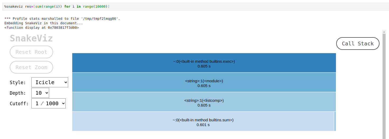
Now we have a nice interactive representation of the time spent in each function, and it is obvious that the summation itself takes the longest. We can choose between two formats of the visualization using ‘Style’ drop-down menu, set the maximum depth of the call stack that is being visualized and set the cutoff value for the functions that won’t be placed on the plot (e.g. by default the functions that take less than 1/1000 of the execution time of the parent function are omitted). By clicking on any of the bars we go deeper into the callstack. Under the plot we have the same statistical table as the cProfile produces. There is also a way to open this visualization in a new browser tab by passing the flag -t after the command.

Other Visualization Tools for cProfile

SnakeViz isn’t the only visualization tool for profiling. You may want to look at the gprof2dot which plots call graphs in the following way, which some users could find more intuitive than the default snakeviz plots:

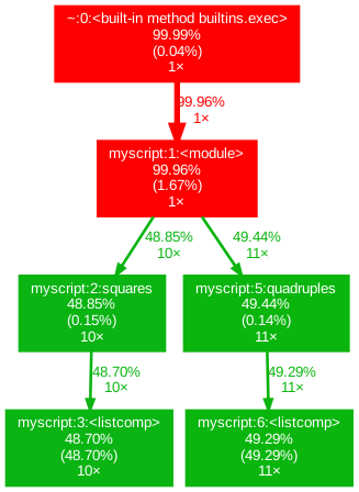
Use SnakeViz to profile the lcanalyzer.calc_stats() function and optimize it for a quicker execution

Apply the %snakeviz to the lcanalyzer.calc_stats() function. Have a look at the output, identify which functions are taking the longest to execute and optimize this code to execute faster.

Solution

After running the following code: %snakeviz calc_stats(lc_dict,bands,'psfMag'), we obtain a visualization that looks similar to this: We can notice that a lot of time is spent in the from_records pandas core function and __getitem__, that is invoked when we use indexing to retrieve some element from a DataFrame. The pandas statistical functions take approximately the same amount of time.

One thing that can be done right away is reducing the number of indexing calls and switching to the numpy statistical functions by converting our data into a numpy.array, e.g. like this:

def calc_stats_nparrs(lc, bands, mag_col):
    # Calculate max, mean and min values for all bands of a light curve
    stats = {}
    for b in bands:
        arr = np.array(lc[b][mag_col])
        stat = {'max':np.max(arr),'mean':np.mean(arr),'min':np.min(arr)}
        stats[b] = stat
    return stats

The profiling result for this function will look like this:

The new version of the function works almost 6 times faster, however, for this we had to change the format of the output. We could have left it as it was, but then the execution time gain would be smaller. With the current changes to the function, we have to rewrite the higher levels of the code and our tests, and, perhaps, rethink in general the data architecture of our software.

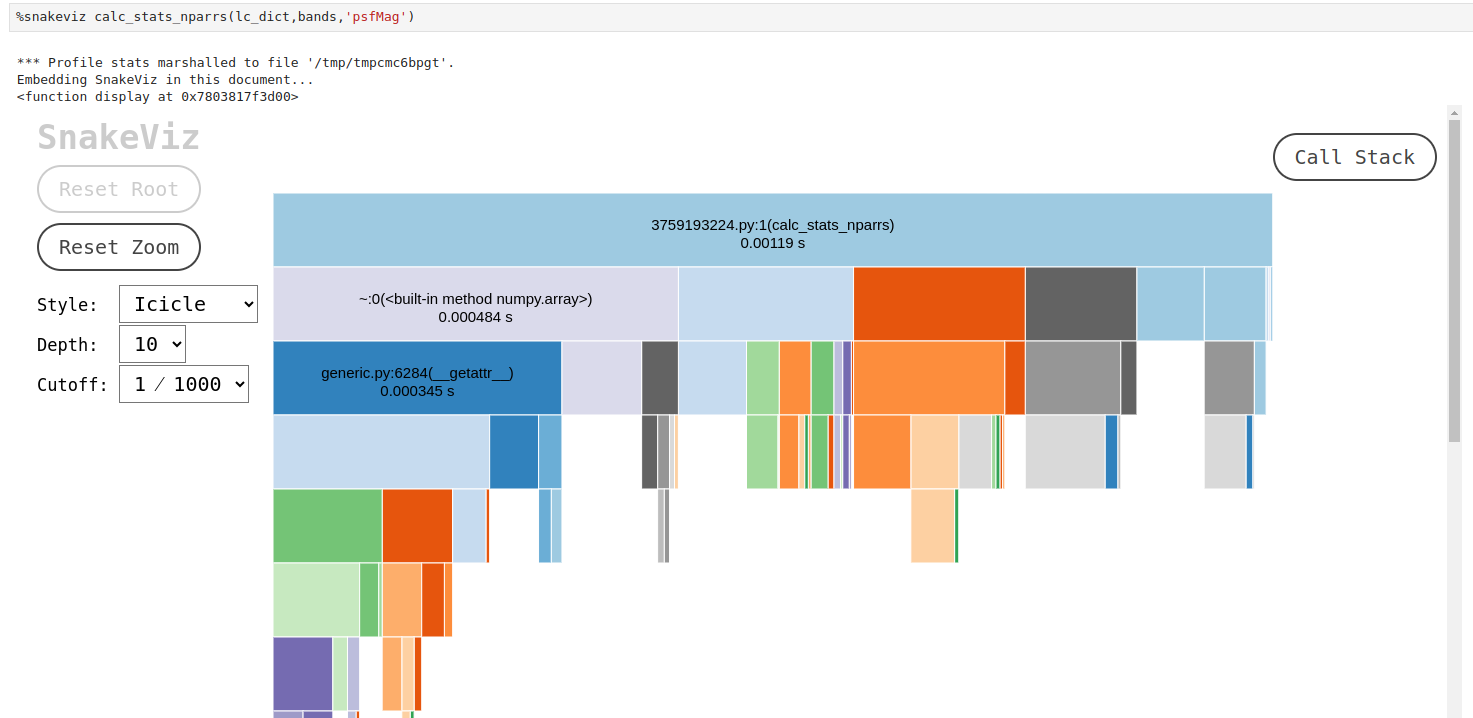
Resource profiling with online profilers

Profiling a running project can be an invaluable tool for identifying and addressing issues, as it catches unusual events that may not be obvious during development. It is possible to do a real-time performance monitoring, although the detailed info on the corresponding instruments goes beyond the scope of today’s workshop. As starting points for further reading, you can have a look at these two repositories:

1. py-spy
2. pyinstrument

Key Points

• For our software to be usable, we need to take care not only of its correctness, but also of its performance.

• Profiling is necessary for large computationally expensive projects or for the software that will be processing large datasets.

• Finding bottlenecks and ineffective subroutines is an important part of refactoring, but it is also a useful thing to do at the stage of planning the architecture of the software.

Verifying Code Style Using Linters

Overview

Teaching: 10 min
Exercises: 5 min

Questions

• What tools can help with maintaining a consistent code style?

• How can we automate code style checking?

Objectives

• Use code linting tools to verify a program’s adherence to a Python coding style convention.

“Any fool can write code that a computer can understand. Good programmers write code that humans can understand.” - Martin Fowler, British software engineer, author and international speaker on software development

Python Coding Style Guide

One of the most important things we can do to make sure our code is readable by others (and ourselves a few months down the line) is to make sure that it is descriptive, cleanly and consistently formatted and uses sensible, descriptive names for variable, function and module names. In order to help us format our code, we generally follow guidelines known as a style guide. A style guide is a set of conventions that we agree upon with our colleagues or community, to ensure that everyone contributing to the same project is producing code which looks similar in style. While a group of developers may choose to write and agree upon a new style guide unique to each project, in practice many programming languages have a single style guide which is adopted almost universally by the communities around the world. In Python, although we do have a choice of style guides available, the PEP 8 style guide is most commonly used. PEP here stands for Python Enhancement Proposals; PEPs are design documents for the Python community, typically specifications or conventions for how to do something in Python, a description of a new feature in Python, etc.

Style consistency

One of the key insights from Guido van Rossum, one of the PEP 8 authors, is that code is read much more often than it is written. Style guidelines are intended to improve the readability of code and make it consistent across the wide spectrum of Python code. Consistency with the style guide is important. Consistency within a project is more important. Consistency within one module or function is the most important. However, know when to be inconsistent - sometimes style guide recommendations are just not applicable. When in doubt, use your best judgment. Look at other examples and decide what looks best. And don’t hesitate to ask!

As we have already covered in the episode on Jupyter Lab IDE, Jupyter Lab highlights the language constructs (reserved words) and syntax errors to help us with coding.

A full list of style guidelines for this style is available from the PEP 8 website. The recommendations regulate indentations, maximum line length, naming of variables, functions and classes, and so on.

Function, Variable, Class, Module, Package Naming in Python

• Function and variable names should use lower_case_with_underscores
• Avoid single character names in almost all instances.
• Variable names should tell you what they store, and not just the type (e.g. source_id is better than string)
• Function names should tell you what the function does.
• Class names should use the CapitalisedWords convention.
• Modules should have short, all-lowercase names. Underscores can be used in the module name if it improves readability.
• Packages should also have short, all-lowercase names, although the use of underscores is discouraged.

A more detailed guide on naming functions, modules, classes and variables is available from PEP8.

Verifying Code Style Using Linters

Knowing the rules of code formatting helps us avoid mistakes during development, so it is always a good idea to dedicate some time to learn how to write PEP8-consistent code from the beginning. However, we also have tools that help us with formatting the already existing code. These tools are called code linters, and their main function is to identify consistency issues in a report-style. Linters analyse source code to identify and report on stylistic and even programming errors. For Jupyter Lab, a number of linters (as well as other tools for improving the quality of your code) are available as part of a package called nbQA. Let’s look at a very well-used one of these called pylint.

First, let’s create a style-fixes git branch to keep our repository organized.

$ git checkout style-fixes

Make sure that you have activated your venv environment, and then install the nbQA package together with the supported tools:

$ python -m pip install -U nbqa
$ python -m pip install -U "nbqa[toolchain]"

We should also update our requirements.txt with this new addition:

$ pip3 freeze > requirements.txt

Using Pylint on the Notebooks

Now we can use Pylint to check the quality of our code. Pylint is a command-line tool that can help our code in many ways:

• Check PEP8 compliance: Pylint will provide a full list of places where your code does not comply with PEP8
• Perform basic error detection: Pylint can look for certain Python type errors
• Check variable naming conventions: Pylint often goes beyond PEP8 to include other common conventions, such as naming variables outside of functions in upper case
• Customisation: you can specify which errors and conventions you wish to check for, and those you wish to ignore

Pylint can also identify code smells.

How Does Code Smell?

There are many ways that code can exhibit bad design whilst not breaking any rules and working correctly. A code smell is a characteristic that indicates that there is an underlying problem with source code, e.g. large classes or methods, methods with too many parameters, duplicated statements in both if and else blocks of conditionals, etc. They aren’t functional errors in the code, but rather are certain structures that violate principles of good design and impact design quality. They can also indicate that code is in need of maintenance and refactoring.

The phrase has its origins in Chapter 3 “Bad smells in code” by Kent Beck and Martin Fowler in Fowler, Martin (1999). Refactoring. Improving the Design of Existing Code. Addison-Wesley. ISBN 0-201-48567-2.

Pylint recommendations are given as warnings or errors, and Pylint also scores the code with an overall mark. We can look at a specific file (e.g. light-curve-analysis.ipynb), or a package (e.g. lcanalyzer). First, let’s look at our notebook:

$ nbqa pylint light-curve-analysis.ipynb --disable=C0114

The output will look somewhat similar to this:

************* Module light-curve-analysis
light-curve-analysis.ipynb:cell_7:3:0: C0301: Line too long (115/100) (line-too-long)
light-curve-analysis.ipynb:cell_1:0:0: C0103: Module name "light-curve-analysis" doesn't conform to snake_case naming style (invalid-name)
light-curve-analysis.ipynb:cell_6:1:0: W0104: Statement seems to have no effect (pointless-statement)
light-curve-analysis.ipynb:cell_1:3:0: W0611: Unused numpy imported as np (unused-import)

-----------------------------------
Your code has been rated at 6.92/10

Your own outputs of the above commands may vary depending on how you have implemented and fixed the code in previous exercises and the coding style you have used.

The five digit codes, such as C0103, are unique identifiers for warnings, with the first character indicating the type of warning. There are five different types of warnings that Pylint looks for, and you can get a summary of them by doing:

$ pylint --long-help

Near the end you’ll see:

  Output:
    Using the default text output, the message format is :
    MESSAGE_TYPE: LINE_NUM:[OBJECT:] MESSAGE
    There are 5 kind of message types :
    * (C) convention, for programming standard violation
    * (R) refactor, for bad code smell
    * (W) warning, for python specific problems
    * (E) error, for probable bugs in the code
    * (F) fatal, if an error occurred which prevented pylint from doing
    further processing.

So for an example of a Pylint Python-specific warning, see the “W0611: Unused numpy imported as np (unused-import)” warning.

Now we can use Pylint for checking our .py files. We can do it in one go, checking the lcanalyzer package at once.

From the project root do:

$ pylint lcanalyzer

Note that this time we use pylint as a standalone, without nbqa, since we are analysing ordinary Python files, not notebooks.

You should see an output similar to the following:

************* Module lcanalyzer
lcanalyzer/__init__.py:1:0: C0304: Final newline missing (missing-final-newline)
************* Module lcanalyzer.models
lcanalyzer/models.py:6:0: C0301: Line too long (107/100) (line-too-long)
lcanalyzer/models.py:41:0: W0105: String statement has no effect (pointless-string-statement)
lcanalyzer/models.py:12:0: W0611: Unused LombScargle imported from astropy.timeseries (unused-import)
************* Module lcanalyzer.views
lcanalyzer/views.py:5:0: C0303: Trailing whitespace (trailing-whitespace)
lcanalyzer/views.py:15:38: C0303: Trailing whitespace (trailing-whitespace)
lcanalyzer/views.py:21:0: C0304: Final newline missing (missing-final-newline)
lcanalyzer/views.py:6:0: C0103: Function name "plotUnfolded" doesn't conform to snake_case naming style (invalid-name)
lcanalyzer/views.py:4:0: W0611: Unused pandas imported as pd (unused-import)

------------------------------------------------------------------
Your code has been rated at 6.09/10 (previous run: 6.09/10, +0.00)

It is important to note that while tools such as Pylint are great at giving you a starting point to consider how to improve your code, they won’t find everything that may be wrong with it.

How Does Pylint Calculate the Score?

The Python formula used is (with the variables representing numbers of each type of infraction and statement indicating the total number of statements):

10.0 - ((float(5 * error + warning + refactor + convention) / statement) * 10)

Note whilst there is a maximum score of 10, given the formula, there is no minimum score - it’s quite possible to get a negative score!

Exercise: Further Improve Code Style of Our Project

Select and fix a few of the issues with our code that Pylint detected. Make sure you do not break the rest of the code in the process and that the code still runs. After making any changes, run Pylint again to verify you’ve resolved these issues.

Make sure you commit and push requirements.txt and any file with further code style improvements you did and merge onto your development and main branches.

$ git add requirements.txt
$ git commit -m "Added Pylint library"
$ git push origin style-fixes
$ git checkout develop
$ git merge style-fixes
$ git push origin develop
$ git checkout main
$ git merge develop
$ git push origin main

Auto-Formatters for the Notebooks

While Pylint provides us with a full report of all kinds of style inconsistencies, most of which have to be fixed manually, some style mistakes can be fixed automatically. For this, we can use black package, also integrated in the nbQA. Save and close your notebook, and then go back to the command line. After running the following command:

$ nbqa black light-curve-analysis.ipynb

Open the notebook again, you will see that black forced line wrap at a certain length of the line, fixed duplicated or missing spaces around parenthesis or commas, aligned elements in the definitions of lists and dictionaries and so on. Using black, you can enforce the same style all over your code and make it much more readable.

Another Way to Use Auto-Formatter

You can use black not only from the command line but from within Jupyter Lab too. For this you will need to install additional extensions, for example, Code Formatter extension. The installation, as usual, can be done using pip:

$ python -m pip install jupyterlab-code-formatter

After that you need to refresh your Jupyter Lab page. In notebook tabs, a new button will appear at the end of the top panel. By clicking this button, you will execute the black formatter over the notebook.

Optional Exercise: Improve Code Style of Your Other Python Projects

If you have a Python project you are working on or you worked on in the past, run it past Pylint to see what issues with your code are detected, if any.

It is possible to automate these kind of code checks with GitHub’s Continuous Integration service GitHub Actions - you can read more on this in the materials of the previous workshops.

Key Points

• Use linting tools in the IDE or on the command line (or via continuous integration) to automatically check your code style.

Wrap-up

Overview

Teaching: 5 min
Exercises: 0 min

Questions

• Looking back at what was covered and how different pieces fit together

• Where are some advanced topics and further reading available?

Objectives

• Put the course in context with future learning.

Further Resources

Below are some additional resources to help you continue learning:

• Intermediate Python for Astronomical Software Development
• InterPython Git Intro
• InterPython Software Testing
• InterPython High-Performance Computing

Key Points

• Maintaining readable and well-structured code is crucial for developing code collaboratively, and for efficient long-term projects.