Resource optimization

Overview

Teaching: 30 min
Exercises: 10 min

Questions

What is the difference between requesting for CPU and GPU resources using Slurm?

How can I optimize my slurm script to avail the best resources for my specific task?

Objectives

Understand different types of computational workloads and their resource requirements

Write optimized Slurm job scripts for sequential, parallel, and GPU workloads

Monitor and analyze resource utilization

Apply best practices for efficient resource allocation

Understanding Resource Requirements

Different computational tasks have varying resource requirements. Understanding these patterns is crucial for efficient HPC usage.

Types of Workloads

CPU-bound workloads: Tasks that primarily use computational power

Mathematical calculations, simulations, data processing
Benefit from more CPU cores and higher clock speeds

Memory-bound workloads: Tasks limited by memory access speed

Large dataset processing, in-memory databases
Require sufficient RAM and fast memory access

I/O-bound workloads: Tasks limited by disk or network operations

File processing, database queries, data transfer
Benefit from fast storage and network connections

GPU-accelerated workloads: Tasks that can utilize parallel processing

Machine learning, scientific simulations, image processing
Require appropriate GPU resources and memory

Types of Jobs and Resources

Job Type	SLURM Partition	Key SLURM Options	Example Use Case
Serial	`serial`	`--partition`, no MPI	Single-thread tensor calc
Parallel	`defaultq`	`-N`, `-n`, `mpirun`	MPI simulation
GPU	`gpu`	`--gpus`, `--cpus-per-task`	Deep learning training

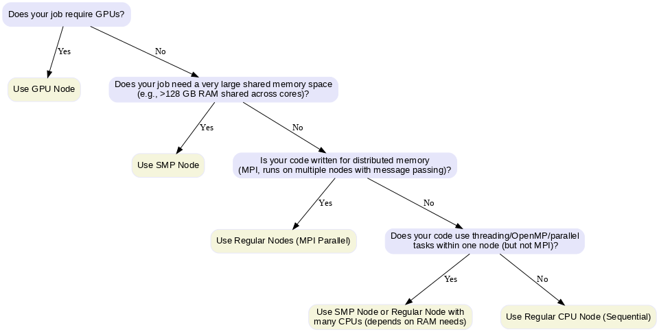
Choosing the Right Node

GPU Node: For massively parallel computations on GPUs (e.g., CUDA, TensorFlow, PyTorch).
SMP Node: For jobs needing large shared memory (big matrices, in-memory data) or multi-threaded code (OpenMP, R, Python multiprocessing).
Regular Node: For MPI-based distributed jobs or simple CPU tasks. Decision chart for Choosing Nodes:

Example

For understanding how we can utilise different resources available on the HPC for the same computational task, we take the example of a python code which calculates the Gravitational Deflection Angle defined in the following way:

Deflection Angle Formula

For light passing near a massive object, the deflection angle (α) in the weak-field approximation is given by:

α = 4GM / (c²b)

Where:

G = Gravitational constant (6.67430 × 10⁻¹¹ m³ kg⁻¹ s⁻²)
M = Mass of the lensing object (in kilograms)
c = Speed of light (299792458 m/s)
b = Impact parameter (the closest approach distance of the light ray to the mass, in meters)

Computational Task Description

Compute the deflection angle over a grid of:

Mass values: From 1 to 1000 solar masses (10³⁰ to 10³³ kg)
Impact parameters: From 10⁹ to 10¹² meters

Generate a 2D array where each entry corresponds to the deflection angle for a specific pair of mass and impact parameter. Now we will look at how we will implement this for the different resources available on the HPC.

Sequential Job Optimization

Sequential jobs run on a single CPU core and are suitable for tasks that cannot be parallelized.

Sequential Job Script Explained

#!/bin/bash
#SBATCH -J jobname                    # Job name for identification
#SBATCH -o outfile.%J                 # Standard output file (%J = job ID)
#SBATCH -e errorfile.%J               # Standard error file (%J = job ID)
#SBATCH --partition=serial            # Use serial queue for single-core jobs
./[programme executable name]          # Execute your program

Script breakdown:

#!/bin/bash: Specifies bash shell for script execution
#SBATCH -J jobname: Sets a descriptive job name for easy identification in queue
#SBATCH -o outfile.%J: Redirects standard output to a file with job ID
#SBATCH -e errorfile.%J: Redirects error messages to separate file
#SBATCH --partition=serial: Specifies the queue/partition for sequential jobs

Example: Gravitational Deflection Angle Sequential CPU

import numpy as np
import time
import matplotlib.pyplot as plt
import os
import matplotlib.colors as colors

# Constants
G = 6.67430e-11
c = 299792458
M_sun = 1.98847e30

# Parameter grid
mass_grid = np.linspace(1, 1000, 10000)  # Solar masses
impact_grid = np.linspace(1e9, 1e12, 10000)  # meters

result = np.zeros((len(mass_grid), len(impact_grid)))

# Timing
start = time.time()

# Sequential computation
for i, M in enumerate(mass_grid):
    for j, b in enumerate(impact_grid):
        result[i, j] = (4 * G * M * M_sun) / (c**2 * b)

end = time.time()

print(f"CPU Sequential time: {end - start:.3f} seconds")

result = np.save("result_cpu.npy", result)
mass_grid = np.save("mass_grid_cpu.npy", mass_grid)
impact_grid = np.save("impact_grid_cpu.npy", impact_grid)

# Load data
result = np.load("result_cpu.npy")
mass_grid = np.load("mass_grid_cpu.npy")
impact_grid = np.load("impact_grid_cpu.npy")

# Create meshgrid
M, B = np.meshgrid(mass_grid / 1.989e30, impact_grid / 1e9, indexing='ij')

# Create output directory
os.makedirs("plots", exist_ok=True)

plt.figure(figsize=(8,6))
pcm = plt.pcolormesh(B, M, result,
                      norm=colors.LogNorm(vmin=result[result > 0].min(), vmax=result.max()),
                      shading='auto', cmap='plasma')

plt.colorbar(pcm, label='Deflection Angle (radians, log scale)')
plt.xlabel('Impact Parameter (Gm)')
plt.ylabel('Mass (Solar Masses)')
plt.title('Gravitational Deflection Angle - CPU')

plt.tight_layout()
plt.savefig("plots/deflection_angle_cpu.png", dpi=300)
plt.close()

print("CPU plot saved in 'plots/deflection_angle_cpu.png'")

Sequential Job Script for the Example

#!/bin/bash
#SBATCH --job-name=HPC_WS_SCPU # Provide a name for the job 
#SBATCH --output=HPC_WS_SCPU_%j.out # Request the output file along with the job number
#SBATCH --error=HPC_WS_SCPU_%j.err # Request the error file along with the job number
#SBATCH --partition=serial
#SBATCH --nodes=1 # Request one CPU node
#SBATCH --ntasks=1 # Request 1 core from the CPU node
#SBATCH --time=-01:00:00 # Set time limit for the job
#SBATCH --mem=16G #Request 16GB memory 

# Load required modules
module purge # Remove the list of pre loaded modules
module load Python/3.9.1
module list

# Create a python virtual environment 
python3 -m venv name_of_your_venv

# Activate your Python environment
source name_of_your_venv/bin/activate

echo "Starting Gravitational Lensing Deflection calculation of Sequential CPU..."
echo "Job ID: $SLURM_JOB_ID"
echo "Node: $SLURM_NODELIST"

# Run the Python script (with logging)
python Gravitational_Deflection_Angle_SCPU.py

echo "Job completed at $(date)"

Exercise: Profile Your Code

Compile and run the sequential code. Use htop to monitor resource usage. Identify whether it’s CPU-bound or memory-bound

Parallel Job Optimization

Parallel jobs can utilize multiple CPU cores across one or more nodes to accelerate computation.

Parallel Job Script Explained

#!/bin/bash
#SBATCH -J jobname                    # Job name
#SBATCH -o outfile.%J                 # Output file
#SBATCH -e errorfile.%J               # Error file
#SBATCH --partition=defaultq          # Parallel job queue
#SBATCH -N 2                          # Number of compute nodes
#SBATCH -n 24                         # Total number of CPU cores per node
mpirun -np 48 ./mpi_program           # Run with 48 MPI processes (2 nodes × 24 cores)

Changes from the sequential script:

#SBATCH --partition=defaultq : Sets to the default partition
#SBATCH -N 2: Requests 2 compute nodes
#SBATCH -n 24: Specifies 24 CPU cores per node
mpirun -np 48: Launches 48 MPI processes total (2 × 24)

Example: Gravitational Deflection Angle Parallel CPU

from mpi4py import MPI
import numpy as np
import time
import os 
import matplotlib.pyplot as plt
import matplotlib.colors as colors

# MPI setup
comm = MPI.COMM_WORLD
rank = comm.Get_rank()
size = comm.Get_size()

# Constants
G = 6.67430e-11
c = 299792458
M_sun = 1.98847e30

# Parameter grid (same on all ranks)
mass_grid = np.linspace(1, 1000, 10000)  # Solar masses
impact_grid = np.linspace(1e9, 1e12, 10000)  # meters

# Distribute mass grid among ranks
chunk_size = len(mass_grid) // size
start_idx = rank * chunk_size
end_idx = (rank + 1) * chunk_size if rank != size - 1 else len(mass_grid)

local_mass = mass_grid[start_idx:end_idx]
local_result = np.zeros((len(local_mass), len(impact_grid)))

# Timing
local_start = time.time()

# Compute local chunk
for i, M in enumerate(local_mass):
    for j, b in enumerate(impact_grid):
        local_result[i, j] = (4 * G * M * M_sun) / (c**2 * b)

local_end = time.time()
print(f"Rank {rank} local time: {local_end - local_start:.3f} seconds")

# Gather results
result = None
if rank == 0:
    result = np.zeros((len(mass_grid), len(impact_grid)))

comm.Gather(local_result, result, root=0)

if rank == 0:
    total_time = local_end - local_start
    print(f"MPI total time (wall time): {total_time:.3f} seconds")
    result = np.save("result_mpi.npy", result)
    mass_grid = np.save("mass_grid_mpi.npy", mass_grid)
    impact_grid = np.save("impact_grid_mpi.npy", impact_grid)

# Load data
result = np.load("result_mpi.npy")
mass_grid = np.load("mass_grid_mpi.npy")
impact_grid = np.load("impact_grid_mpi.npy")

# Create meshgrid
M, B = np.meshgrid(mass_grid / 1.989e30, impact_grid / 1e9, indexing='ij')

# Create output directory
os.makedirs("plots", exist_ok=True)

plt.figure(figsize=(8,6))
pcm = plt.pcolormesh(B, M, result,
                      norm=colors.LogNorm(vmin=result[result > 0].min(), vmax=result.max()),
                      shading='auto', cmap='plasma')

plt.colorbar(pcm, label='Deflection Angle (radians, log scale)')
plt.xlabel('Impact Parameter (Gm)')
plt.ylabel('Mass (Solar Masses)')
plt.title('Gravitational Deflection Angle - MPI')

plt.tight_layout()
plt.savefig("plots/deflection_angle_mpi.png", dpi=300)
plt.close()

print("MPI plot saved in 'plots/deflection_angle_mpi.png'")

Parallel Job Script for the Example

#!/bin/bash
#SBATCH --job-name=HPC_WS_PCPU # Provide a name for the job 
#SBATCH --output=HPC_WS_PCPU_%j.out # Request the output file along with the job number
#SBATCH --error=HPC_WS_PCPU_%j.err # Request the error file along with the job number
#SBATCH --partition=defaultq 
#SBATCH --nodes=2 # Request two CPU nodes
#SBATCH --ntasks=4 # Request 2 cores from each CPU node
#SBATCH --time=-01:00:00 # Set time limit for the job
#SBATCH --mem=16G #Request 16GB memory 

# Load required modules
module purge # Remove the list of pre loaded modules
module load Python/3.9.1
module load openmpi4/default
module list # List the modules

# Create a python virtual environment 
python3 -m venv name_of_your_venv

# Activate your Python virtual environment
source name_of_your_venv/bin/activate

echo "Starting Gravitational Lensing Deflection calculation of Sequential CPU..."
echo "Job ID: $SLURM_JOB_ID"
echo "Node: $SLURM_NODELIST"

# Run the Python script with MPI (with logging)
mpirun -np 4 python Gravitational_Lensing_PCPU.py

echo "Job completed at $(date)"

Exercise: Optimize Parallel Performance

Compile the OpenMP version with different thread counts. Submit jobs with varying --cpus-per-task values. Plot performance vs. thread count

GPU Job Optimization

GPU jobs leverage graphics processing units for massively parallel computations.

GPU Job Script Explained

#!/bin/bash
#SBATCH --nodes=1                     # Single node (GPUs are node-local)
#SBATCH --ntasks-per-node=1           # One task per node
#SBATCH --cpus-per-task=4             # CPU cores to support GPU
#SBATCH -o output-%J.out              # Output file with job ID
#SBATCH -e error-%J.err               # Error file with job ID
#SBATCH --partition=gpu               # GPU-enabled partition
#SBATCH --mem 32G                     # Memory allocation
#SBATCH --gpus-per-node=1             # Number of GPUs requested
./[programme executable name]          # GPU program execution

GPU-specific parameters:

--partition=gpu: Specifies GPU-enabled compute nodes
--gpus-per-node=1: Requests one GPU per node
--mem 32G: Allocates sufficient memory for GPU operations
--cpus-per-task=4: Provides CPU cores to feed data to GPU

Example: CUDA Implementation

import numpy as np
from numba import cuda
import time
import matplotlib.pyplot as plt
import os
import matplotlib.colors as colors


# Constants
G = 6.67430e-11
c = 299792458

# Parameter grid
mass_grid = np.linspace(1e30, 1e33, 10000)
impact_grid = np.linspace(1e9, 1e12, 10000)

mass_grid_device = cuda.to_device(mass_grid)
impact_grid_device = cuda.to_device(impact_grid)
result_device = cuda.device_array((len(mass_grid), len(impact_grid)))

# CUDA kernel
@cuda.jit
def compute_deflection(mass_array, impact_array, result):
    i, j = cuda.grid(2)
    if i < mass_array.size and j < impact_array.size:
        M = mass_array[i]
        b = impact_array[j]
        result[i, j] = (4 * G * M) / (c**2 * b)

# Setup thread/block dimensions
threadsperblock = (16, 16)
blockspergrid_x = (mass_grid.size + threadsperblock[0] - 1) // threadsperblock[0]
blockspergrid_y = (impact_grid.size + threadsperblock[1] - 1) // threadsperblock[1]
blockspergrid = (blockspergrid_x, blockspergrid_y)

# Run the kernel
start = time.time()
compute_deflection[blockspergrid, threadsperblock](mass_grid_device, impact_grid_device, result_device)
cuda.synchronize()
end = time.time()

result = result_device.copy_to_host()

print(f"CUDA time: {end - start:.3f} seconds")

# Save the result and grids
np.save("result_cuda.npy", result)
np.save("mass_grid_cuda.npy", mass_grid)
np.save("impact_grid_cuda.npy", impact_grid)

print("Result and grids saved as .npy files.")

# Load data
result = np.load("result_cuda.npy")
mass_grid = np.load("mass_grid_cuda.npy")
impact_grid = np.load("impact_grid_cuda.npy")

# Create meshgrid
M, B = np.meshgrid(mass_grid / 1.989e30, impact_grid / 1e9, indexing='ij')

# Create output directory
os.makedirs("plots", exist_ok=True)

plt.figure(figsize=(8,6))
pcm = plt.pcolormesh(B, M, result,
                      norm=colors.LogNorm(vmin=result[result > 0].min(), vmax=result.max()),
                      shading='auto', cmap='plasma')

plt.colorbar(pcm, label='Deflection Angle (radians, log scale)')
plt.xlabel('Impact Parameter (Gm)')
plt.ylabel('Mass (Solar Masses)')
plt.title('Gravitational Deflection Angle - CUDA')

plt.tight_layout()
plt.savefig("plots/deflection_angle_cuda.png", dpi=300)
plt.close()

print("CUDA plot saved in 'plots/deflection_angle_cuda.png'")

GPU Job Script for the Example

#!/bin/bash
#SBATCH --job-name=HPC_WS_GPU  # Provide a name for the job 
#SBATCH --output=HPC_WS_GPU_%j.out
#SBATCH --error=HPC_WS_GPU_%j.err
#SBATCH --partition=gpu
#SBATCH --nodes=1
#SBATCH --ntasks-per-node=1
#SBATCH --cpus-per-task=4 # Number of CPUs for data preparation 
#SBATCH --mem=32G # Memmory allocation
#SBATCH --gpus-per-node=1
#SBATCH --time=06:00:00

# --------- Load Environment ---------
module load Python/3.9.1
module load cuda/11.2
module list

# Activate your Python virtual environment
source name_of_your_venv/bin/activate

# --------- Run the Python Script ---------
python Gravitational_Lensing_GPU.py

Exercise: GPU vs CPU Comparison

Run the tensor operations script on both CPU and GPU. Compare execution times and memory usage. Calculate the speedup factor

Resource Monitoring and Performance Analysis

Monitoring Job Performance

#!/bin/bash

#SBATCH --partition=gpu
#SBATCH --gpus=1
#SBATCH --job-name=ResourceMonitor
#SBATCH --output=ResourceMonitor_%j.out
#SBATCH --time=00:10:00  # 10 minutes max (5 for monitoring + buffer)

# --------- Configuration ---------
LOG_FILE="resource_monitor.log"
INTERVAL=30    # Interval between logs in seconds
DURATION=60   # Total duration in seconds (5 minutes)
ITERATIONS=$((DURATION / INTERVAL))

# --------- Start Monitoring ---------
echo "Starting Resource Monitoring for $DURATION seconds (~$((DURATION/60)) minutes)..."
echo "Logging to: $LOG_FILE"
echo "------ Monitoring Started at $(date) ------" >> "$LOG_FILE"

# --------- System Info Check ---------
echo "==== System Info Check ====" | tee -a "$LOG_FILE"
echo "Hostname: $(hostname)" | tee -a "$LOG_FILE"

# Check NVIDIA driver and GPU presence
if command -v nvidia-smi &> /dev/null; then
    echo "✅ nvidia-smi is available." | tee -a "$LOG_FILE"
    if nvidia-smi &>> "$LOG_FILE"; then
        echo "✅ GPU detected and driver is working." | tee -a "$LOG_FILE"
    else
        echo "⚠️ NVIDIA-SMI failed. Check GPU node or driver issues." | tee -a "$LOG_FILE"
    fi
else
    echo "❌ nvidia-smi is not installed." | tee -a "$LOG_FILE"
fi

echo "Checking for NVIDIA GPU presence on PCI bus..." | tee -a "$LOG_FILE"
if lspci | grep -i nvidia &>> "$LOG_FILE"; then
    echo "✅ NVIDIA GPU found on PCI bus." | tee -a "$LOG_FILE"
else
    echo "❌ No NVIDIA GPU detected on this node." | tee -a "$LOG_FILE"
fi

echo "" | tee -a "$LOG_FILE"

# --------- Trap CTRL+C for Clean Exit ---------
trap "echo 'Stopping monitoring...'; echo '------ Monitoring Ended at $(date) ------' >> \"$LOG_FILE\"; exit" SIGINT SIGTERM

# --------- Monitoring Loop ---------
for ((i=1; i<=ITERATIONS; i++)); do
    echo "========================== $(date) ==========================" >> "$LOG_FILE"

    # GPU usage monitoring
    echo "--- GPU Usage (nvidia-smi) ---" >> "$LOG_FILE"
    nvidia-smi 2>&1 | grep -v "libnvidia-ml.so" >> "$LOG_FILE"
    echo "" >> "$LOG_FILE"

    # CPU and Memory monitoring
    echo "--- CPU and Memory Usage (top) ---" >> "$LOG_FILE"
    top -b -n 1 | head -20 >> "$LOG_FILE"
    echo "" >> "$LOG_FILE"

    sleep $INTERVAL
done

echo "------ Monitoring Ended at $(date) ------" >> "$LOG_FILE"
echo "✅ Resource monitoring completed."

Understanding Outputs - `top` - CPU and Memory Monitoring

Example Output:

--- CPU and Memory Usage (top) ---
top - 17:53:49 up 175 days,  9:41,  0 users,  load average: 1.01, 1.06, 1.08
Tasks: 765 total,   1 running, 764 sleeping,   0 stopped,   0 zombie
%Cpu(s):  2.2 us,  0.1 sy,  0.0 ni, 97.7 id,  0.0 wa,  0.0 hi,  0.0 si,  0.0 st
MiB Mem : 515188.2 total, 482815.2 free,  17501.5 used,  14871.5 buff/cache
MiB Swap:   4096.0 total,   4072.2 free,     23.8 used. 493261.3 avail Mem

Explanation:

Header Line - System Uptime and Load Average

top - 17:53:49 up 175 days,  9:41,  0 users,  load average: 1.01, 1.06, 1.08

17:53:49 - Current time.
up 175 days, 9:41 - How long the system has been running.
0 users - Number of users logged in.
load average - System load over 1, 5, and 15 minutes.
- A load of 1.00 means one CPU core is fully utilized.

Task Summary

Tasks: 765 total,   1 running, 764 sleeping,   0 stopped,   0 zombie

765 total - Total processes.
1 running - Actively running.
764 sleeping - Waiting for input or tasks.
0 stopped - Stopped processes.
0 zombie - Zombie processes (defunct).

CPU Usage

%Cpu(s):  2.2 us,  0.1 sy,  0.0 ni, 97.7 id,  0.0 wa,  0.0 hi,  0.0 si,  0.0 st

Field	Meaning
us	User CPU time - 2.2%
sy	System (kernel) time - 0.1%
ni	Nice (priority) - 0.0%
id	Idle - 97.7%
wa	Waiting for I/O - 0.0%
hi	Hardware interrupts - 0.0%
si	Software interrupts - 0.0%
st	Steal time (virtualization) - 0.0%

Memory Usage

MiB Mem : 515188.2 total, 482815.2 free,  17501.5 used,  14871.5 buff/cache

Field	Meaning
total	Total RAM (515188.2 MiB)
free	Free RAM (482815.2 MiB)
used	Used by programs (17501.5 MiB)
buff/cache	Disk cache and buffers (14871.5 MiB)

Swap Usage

MiB Swap:   4096.0 total,   4072.2 free,     23.8 used. 493261.3 avail Mem

Field	Meaning
total	Swap space available (4096 MiB)
free	Free swap (4072.2 MiB)
used	Swap used (23.8 MiB)
avail Mem	Available memory for new tasks (493261.3 MiB)

These explanations cover the descriptions of each of the different parameters given by the top output.

Understanding Outputs - `nvidia-smi` GPU Monitoring

Example `nvidia-smi` Output:

------ Wed Jul  2 17:12:23 IST 2025 ------
Wed Jul  2 17:12:23 2025       
+-----------------------------------------------------------------------------------------+
| NVIDIA-SMI 560.35.05              Driver Version: 560.35.05      CUDA Version: 12.6     |
|-----------------------------------------+------------------------+----------------------|
| GPU  Name                 Persistence-M | Bus-Id          Disp.A | Volatile Uncorr. ECC |
| Fan  Temp   Perf          Pwr:Usage/Cap |           Memory-Usage | GPU-Util  Compute M. |
|                                         |                        |               MIG M. |
|=========================================+========================+======================|
|   0  NVIDIA H100 NVL                On  |   00000000:AB:00.0 Off |                    0 |
| N/A   37C    P0             86W /  400W |    1294MiB /  95830MiB |      0%      Default |
|                                         |                        |             Disabled |
+-----------------------------------------+------------------------+----------------------+
                                                                                         
+-----------------------------------------------------------------------------------------+
| Processes:                                                                              |
|  GPU   GI   CI        PID   Type   Process name                              GPU Memory |
|        ID   ID                                                               Usage      |
|=========================================================================================|
|    0   N/A  N/A   2234986      C   python                                       1284MiB |
+-----------------------------------------------------------------------------------------+

…

Explanation of `nvidia-smi` Output:

GPU Summary Header

NVIDIA-SMI Version: 560.35.05 — Monitoring tool version.
Driver Version: 560.35.05 — NVIDIA driver version installed.
CUDA Version: 12.6 — CUDA toolkit compatibility version.

GPU Info Section

Field	Meaning
GPU	GPU index number (0)
Name	GPU model: NVIDIA H100 NVL
Persistence-M	Persistence Mode: On (reduces init overhead)
Bus-Id	PCI bus ID location
Disp.A	Display Active: Off (no display connected)
Volatile Uncorr. ECC	GPU memory error count (0 = no errors)
Fan	Fan speed (N/A — passive cooling)
Temp	Temperature (37C — healthy)
Perf	Performance state (P0 = maximum performance)
Pwr:Usage/Cap	Power usage (86W of 400W max)
Memory-Usage	1294MiB used / 95830MiB total
GPU-Util	GPU utilization (0% — idle)
Compute M.	Compute mode (Default)
MIG M.	Multi-Instance GPU mode (Disabled)

Processes Section

Field	Meaning
GPU	GPU ID (0)
PID	Process ID (2234986)
Type	Type of process: C (compute)
Process Name	Process name (python)
GPU Memory	1284MiB used by this process

These explanations cover the descriptions of each of the different parameters given by the nvidia-smi output.

Performance Comparison Script

import matplotlib.pyplot as plt

# Extracted timings from the printed output
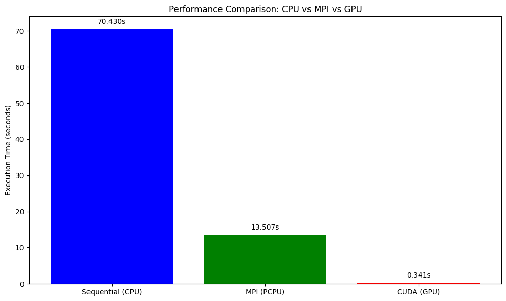
methods = ['Sequential (CPU)', 'MPI (PCPU)', 'CUDA (GPU)']
times = [70.430, 13.507, 0.341] # Replace the times with the times printed by running the above scripts

plt.figure(figsize=(10, 6))
bars = plt.bar(methods, times, color=['blue', 'green', 'red'])
plt.ylabel('Execution Time (seconds)')
plt.title('Performance Comparison: CPU vs MPI vs GPU')

# Add labels above bars
for bar, time in zip(bars, times):
    plt.text(bar.get_x() + bar.get_width() / 2, bar.get_height() + 1,
             f'{time:.3f}s', ha='center', va='bottom')

plt.tight_layout()
plt.savefig('performance_comparison.png', dpi=300, bbox_inches='tight')
plt.show()

Exercise: Resource Efficiency Analysis

Run the above python script to create a comparitive analysis between the different methods you used in this tutorial to understand the efficiency of different resources

Example Solution

This plot shows the execution time comparison between CPU, MPI, and GPU implementations.

Best Practices and Common Pitfalls

Resource Allocation Best Practices

Match resources to workload requirements
- Don’t request more resources than you can use
- Consider memory requirements carefully
- Use appropriate partitions/queues
Test with small jobs first
- Validate your scripts with shorter runs
- Check resource utilization before scaling up
Monitor and optimize
- Use profiling tools to identify bottlenecks
- Adjust resource requests based on actual usage

Common Mistakes to Avoid

Over-requesting resources

# Bad: Requesting 32 cores for sequential code
#SBATCH --cpus-per-task=32
./sequential_program
   
# Good: Match core count to parallelization
#SBATCH --cpus-per-task=1
./sequential_program

Memory allocation errors

# Bad: Not specifying memory for memory-intensive jobs
#SBATCH --partition=defaultq
   
# Good: Specify adequate memory
#SBATCH --partition=defaultq
#SBATCH --mem=16G

GPU job inefficiencies

# Bad: Too many CPU cores for GPU job
#SBATCH --cpus-per-task=32
#SBATCH --gpus-per-node=1
   
# Good: Balanced CPU-GPU ratio
#SBATCH --cpus-per-task=4
#SBATCH --gpus-per-node=1

Summary

Resource optimization in HPC involves understanding your workload characteristics and matching them with appropriate resource allocations. Key takeaways:

Profile your code to understand resource requirements
Use sequential jobs for single-threaded applications
Leverage parallel computing for scalable workloads
Utilize GPUs for massively parallel computations
Monitor performance and adjust allocations accordingly
Avoid common pitfalls like over-requesting resources

Efficient resource utilization not only improves your job performance but also ensures fair access to shared HPC resources for all users.

Revisit Earlier Exercises

Now that you’ve learned how to submit jobs using Slurm and request computational resources effectively, revisit the following exercises from the earlier lesson:

Exercise: MPI using mpi4py

Exercise: GPU vector addition with numba-cuda

Try running them now on your cluster using the appropriate Slurm script and resource flags.

Solution 1: Slurm Submission Script for Exercise MPI with mpi4py

The following script can be used to submit your MPI-based Python program (mpi_hpc_ws.py) on an HPC cluster using Slurm:
#!/bin/bash
#SBATCH --job-name=mpi_hpc_ws
#SBATCH --output=mpi_%j.out
#SBATCH --error=mpi_%j.err
#SBATCH --partition=defaultq
#SBATCH --nodes=2
#SBATCH --ntasks=4
#SBATCH --time=00:10:00
#SBATCH --mem=16G

# Load required modules
module purge
module load Python/3.9.1
module list


Create a python virtual environment 
python3 -m venv name_of_your_venv

Activate your Python environment
source name_of_your_venv/bin/activate

# Run the MPI job
mpirun -np 4 python mpi_hpc_ws.py
Make sure your virtual environment has mpi4py installed and that your system has access to the OpenMPI runtime via mpirun. Adjust the number of nodes and tasks depending on the cluster policies.

Solution 2: Slurm Submission Script for Exercise GPU with `numba-cuda`

The following script can be used to submit a GPU-accelerated Python job (numba_cuda_test.py) using Slurm:

#!/bin/bash
#SBATCH --job-name=Numba_Cuda
#SBATCH --output=Numba_Cuda_%j.out
#SBATCH --error=Numba_Cuda_%j.err
#SBATCH --partition=gpu
#SBATCH --nodes=1
#SBATCH --ntasks-per-node=1
#SBATCH --cpus-per-task=4
#SBATCH --mem=16G
#SBATCH --gpus-per-node=1
#SBATCH --time=00:10:00

# --------- Load Environment ---------
module load Python/3.9.1
module load cuda/11.2
module list

# --------- Check whether the GPU is available ---------
from numba import cuda
print("CUDA Available:", cuda.is_available())
# Activate virtual environment
source 'name_of_venv'/bin/activate # Here name_of_venv refers to the name of your virtual environment without the quotes

# --------- Run the Python Script ---------
python numba_cuda_test.py

Make sure your virtual environment includes the numba-cuda python library to access the GPU.

Key Points

Different computational models (sequential, parallel, GPU) significantly impact runtime and efficiency.

Sequential CPU execution is simple but inefficient for large parameter spaces.

Parallel CPU (e.g., MPI or OpenMP) reduces runtime by distributing tasks but is limited by CPU core counts and communication overhead.

GPU computing can drastically accelerate tasks with massively parallel workloads like grid-based simulations.

Choosing the right computational model depends on the problem structure, resource availability, and cost-efficiency.

Effective Slurm job scripts should match the workload to the hardware: CPUs for serial/parallel, GPUs for highly parallelizable tasks.

Monitoring tools (like nvidia-smi, seff, top) help validate whether the resource request matches the actual usage.

Optimizing resource usage minimizes wait times in shared environments and improves overall throughput.

previous episode

Introduction to High Performance Computing for astronomical software development

next episode