Setting the Scene
Overview
Teaching: 10 min
Exercises: 0 minQuestions
What are we teaching in this course?
To whom will this course be useful?
Objectives
Setting the scene and expectations
Making sure everyone has all the necessary software installed
Introduction
Astronomy has always been a data-hungry field. From the discovery of Neptune to state-of-the-art cosmological simulations, such as Illustris or FLAMINGO, we make discoveries by working with datasets that push the limits of our processing capabilities, and sometimes exceed them. To handle gigabytes of observations or millions of simulated particles, we must optimize our code as much as possible, pay close attention to how we use available RAM and processors, and eventually turn to more powerful computers than we can fit on our desks.
In this course, we provide an introduction to High-Performance Computing — a set of approaches and techniques for using supercomputers and computer clusters. While modern HPC facilities are often built from the same components as “ordinary” PCs and can run your code with minimal adjustments, careful planning is required to avoid bottlenecks such as data transfer between nodes and to take full advantage of massive parallelization.
A full course on High-Performance Computing would take many hours of lectures and practical exercises. Here, over the next two days, we will cover the basics of the field and practice what we’ve learned on one of the LSST HPC facilities, the Croatian supercomputer Bura.
The course is organised into the following sections:
Section 1: HPC Intro
On day 1, we will do a general overview of what is considered to be HPC, which approaches for speeding up your software exist, and how to understand whether your algorithm will work faster if you try to run it on a cluster or supercomputer. After a brief refresher on Command line usage, we are also going to get familiar with the Bura supercomputer and learn about one of the most common job manager tools called Slurm.
Section 2: Running and adapting your code to HPC
The second-day episodes are dedicated to running code examples on Bura and studying how various implementations utilise the resources available in an HPC environment. We will compare code performance when it is run on a single CPU, multiple CPUs or GPUs, how different parallelization instruments work, and learn how to use resource management tools for determining which aspects of your algorithm require further improvements.
Before We Start
A few notes before we start.
Prerequisite Knowledge
This is an intermediate-level software development course intended for people who have already been developing code in Python (or other languages) and applying it to their own problems after gaining basic software development skills. So, it is expected that you have some prerequisite knowledge on the topics covered, such as Python imports, variables, and loops, virtual environments, and executing commands in your OS terminal. While we attempted to make the materials clear and understandable to a wide range of expertise levels, if you are not familiar with Python and the command line, we recommend that you e.g. go through one of the entry levels Carpentries workshops, such as Programming with Python.
Setup, Common Issues & Fixes
Have you setup and installed all the tools and accounts required for this course? Check the list of common issues, fixes & tips if you experience any problems running any of the tools you installed - your issue may be solved there.
Compulsory and Optional Exercises
Exercises are a crucial part of this course and the narrative. They are used to reinforce the points taught and give you an opportunity to practice things on your own. Please do not be tempted to skip exercises as that will get your local software project out of sync with the course and break the narrative. Exercises that are clearly marked as “optional” can be skipped without breaking things but we advise you to go through them too, if time allows.
Outdated Screenshots
Throughout this lesson we will make use and show content from various interfaces, e.g. websites, PC-installed software, command line, etc. These are evolving tools and platforms, always adding new features and new visual elements. Screenshots in the lesson may then become out-of-sync, refer to or show content that no longer exists or is different to what you see on your machine. If during the lesson you find screenshots that no longer match what you see or have a big discrepancy with what you see, please open an issue describing what you see and how it differs from the lesson content. Feel free to add as many screenshots as necessary to clarify the issue.
Let Us Know About the Issues
The materials were prepared specifically for this workshop. They weren’t used before, and there may be typos, code errors, or underexplained or unclear moments. Please, let us know about these issues. It will help us to improve the materials and make the next workshop better.
Key Points
Astronomical research requires large computing resources, which are not always available within a PC form-factor.
In order to run your code in a High-Performance Computing setting, special tools and techniques are needed.
Section 1: HPC basics
Overview
Teaching: 5 min
Exercises: 0 minQuestions
What are the topics covered in Section 1?
Objectives
To overview the topics of the Section 1.
This section covers the introduction to HPC computing:
- What is HPC, what is parallelization, which types of parallelization exist and how it’s connected to the computer and network architectures?
- What kinds of HPC are available in the astronomical community in general and in LSST network in particular?
- How do we access HPC Bura and what resources are available there?
- How to use the command line for executing our code on a remote computer?
- How to set up the virtual environment and use Python on Bura?
- What is workload manager, how resources are allocated in an HPC setting, and how to use Slurm?
Key Points
The topics covered in this section are HPC intro, Bura HPC facility and Slurm workload manager.
HPC Intro
Overview
Teaching: 20 min
Exercises: 0 minQuestions
What is sequential and parallel code execution?
How do computer and network architecture define computational performance for personal and supercomputers?
What types of parallelization exist?
How data storage works in HPC?
Objectives
To learn how computer and network architecture affect performance.
To understand how HPC facilities are organized.
Simple, inexpensive computing tasks are typically performed sequentially, i.e., instructions are executed one after another in the order they appear in the code. This is the default paradigm in most programming languages. For larger problems that involve many tasks, it is often more efficient to exploit the intrinsically parallel nature of modern processors, which are designed to execute multiple processes simultaneously. Many programming languages, including Python, support parallel execution, where multiple CPU cores perform tasks independently.
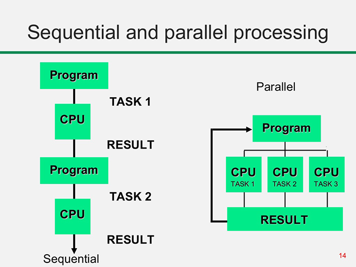
Figure 1: Illustration of sequential vs. parallel processing. Credit: https://itrelease.com/2017/11/difference-serial-parallel-processing/
As computational demands grow, parallel programming has become increasingly essential. From protein folding in drug discovery to simulations of galaxy formation and evolution, many complex problems in science rely on parallel computing. Parallel programming, hardware architecture, and systems administration intersect in the multidisciplinary field of high-performance computing (HPC). Unlike running code locally on a personal computer, HPC typically involves connecting to a cluster of networked computers, sometimes located all over the world, designed to work together on large-scale tasks.
The efficiency of a supercomputer in application to different tasks depends not only on the number of processors it carries aboard, but also on its architecture (or, in case of a cluster, on the network architecture). In this episode, we’ll briefly consider the terminology and classifications used to describe supercomputers of different types.
Computer Architectures
Historically, computer architectures are often classified into two categories: von Neumann and Harvard.
In the von Neumann design, a computer system contains the following components:
- Arithmetic/logic unit (ALU)
- Control unit (CU)
- Memory unit (MU)
- Input/output (I/O) devices
The ALU retrieves data from the MU and performs calculations, while the CU interprets instructions and directs the flow of data to and from the I/O devices, as shown in the diagram below.
In this architecture, the MU stores both data and instructions, which creates a performance bottleneck due to limited data transfer bandwidth, commonly referred to as the von Neumann bottleneck.
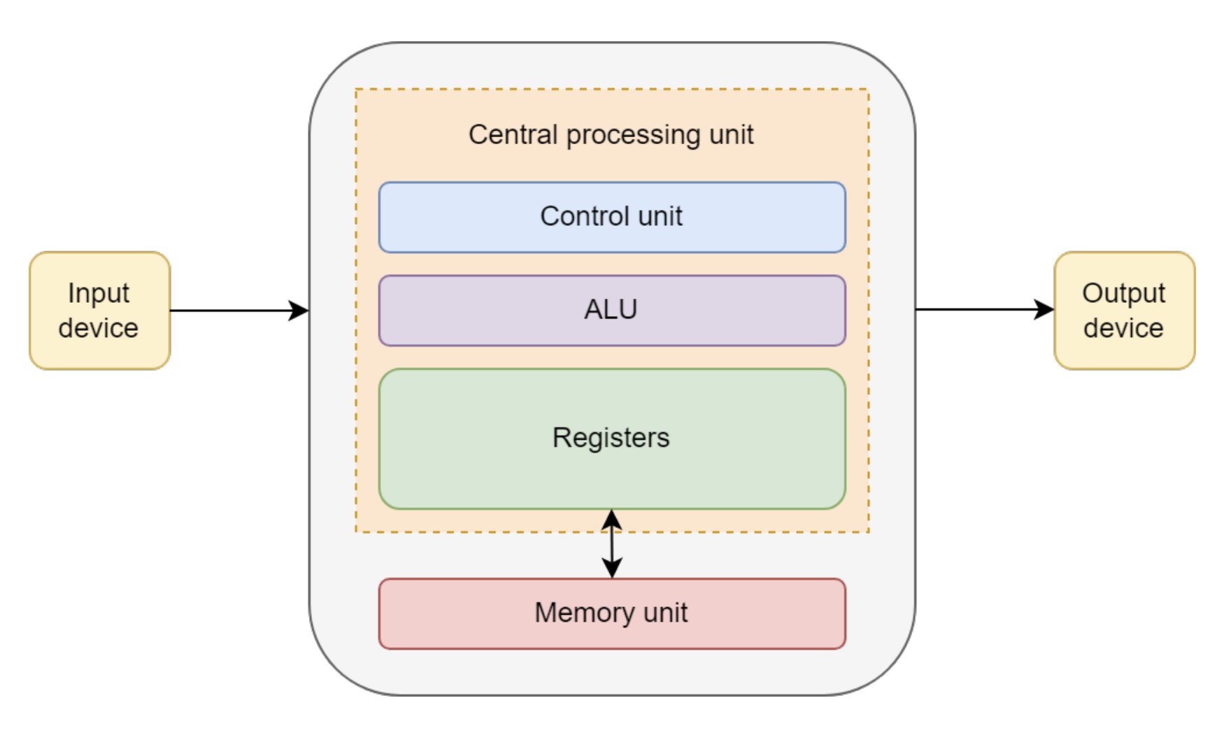
Figure 2: Diagram of von Neumann architecture, from https://onlinelibrary.wiley.com/doi/book/10.1002/9780470932025
The Harvard architecture is a variant of the von Neumann design in which instruction and data storage are physically separated.
This allows simultaneous access to both instructions and data, partially overcoming the von Neumann bottleneck.
Most modern central processing units (CPUs) use a modified Harvard architecture, in which instructions and data have separate caches but share the same main memory.
This hybrid approach combines some of the performance benefits of Harvard with the flexibility of von Neumann.
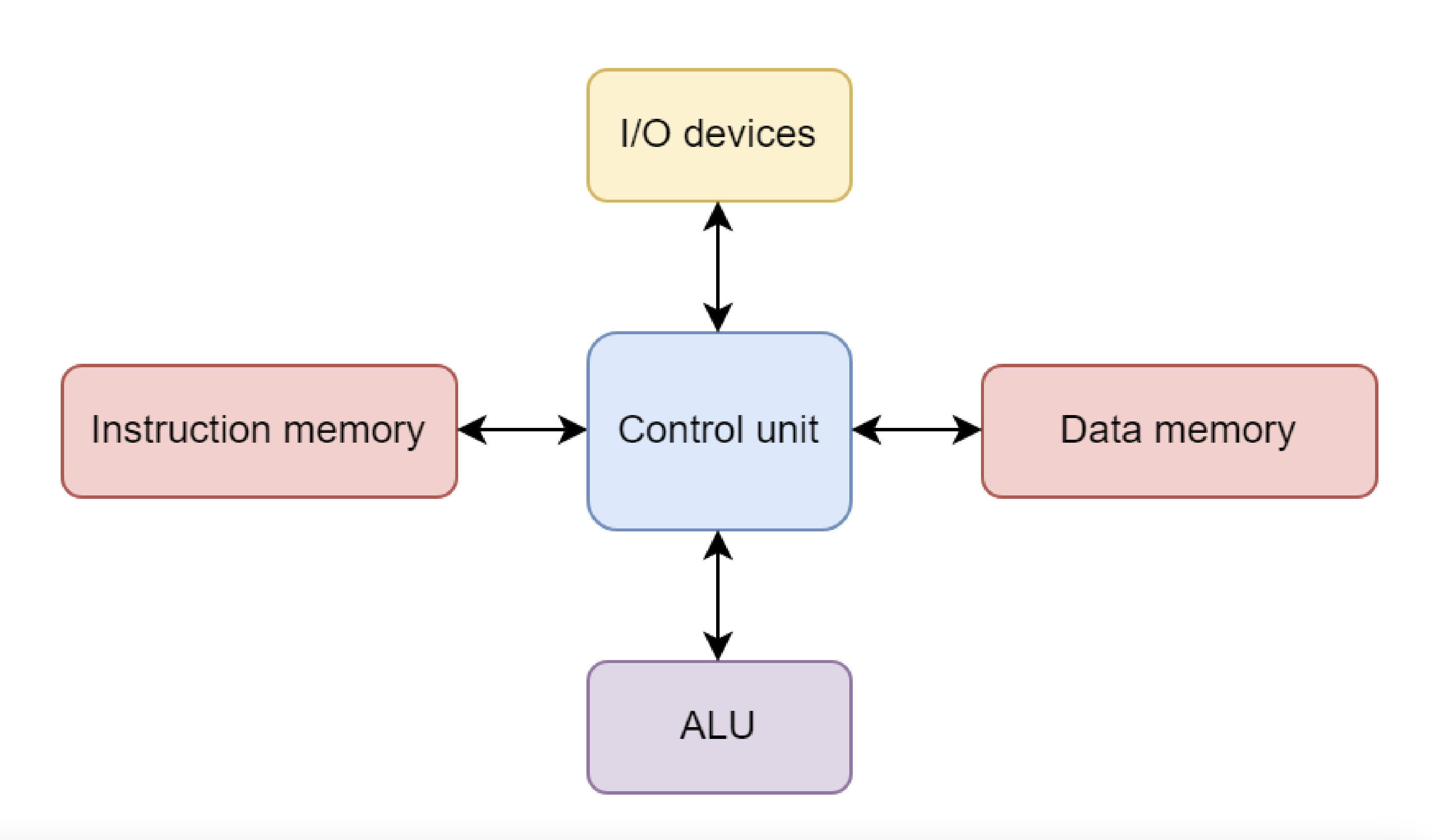
Figure 3: Diagram of Harvard architecture, from https://onlinelibrary.wiley.com/doi/book/10.1002/9780470932025
Performance
Three main components have the greatest impact on computational performance:
-
CPU: CPU performance is often quantified by frequency, or “clock speed,” which determines how quickly a CPU executes instructions in terms of cycles per second. For example, a CPU with a clock speed of 3.5 GHz performs 3.5 billion cycles each second. Many CPUs have multiple cores, enabling parallel execution of multiple instructions simultaneously (Intel).
-
RAM: Random access memory (RAM) is a computer’s short-term memory, storing the data needed to run applications and open files. Faster RAM allows data to move to and from the CPU more quickly, and larger RAM capacity enables the CPU to handle more complex operations simultaneously (Intel).
-
Hard drive: In contrast to RAM, a computer’s hard drive is used for long-term data storage. Hard drives are characterized by both their capacity and performance. Higher-capacity drives can store more data, while higher-performance drives can read and write data faster. Hard disk drives (HDDs) generally offer more capacity for a lower cost, whereas solid state drives (SSDs) provide better performance and reliability.
Processing astronomical data, building models, and running simulations requires significant computational power. The laptop or PC you are using right now likely has between 8 GB and 32 GB of RAM, a processor with 4–10 cores, and a hard drive that can store 256 GB–1 TB of data. But what if you need to process a dataset larger than 1 TB, or load a model into RAM that exceeds 32 GB, or run a simulation that would take a month to complete on your CPU? In that case, you need a bigger computer or many computers working in parallel.
Flynn’s Taxonomy: A Framework for Parallel Computing
When discussing parallel computing, it is helpful to have a framework for classifying different types of computer architectures. The most widely used is Flynn’s Taxonomy, proposed in 1966 (Flynn, 1966). It provides a simple vocabulary for describing how computers handle tasks and will help us understand why certain programming models are better suited to certain problems.
Flynn’s taxonomy is based on four terms:
- Single
- Instruction
- Multiple
- Data
These combine to define four main architectures (HiPowered book):
- SISD (Single Instruction, Single Data): A traditional serial computer, also called a von Neumann machine. It executes one instruction at a time on a single piece of data. A laptop running a simple, non-parallel program is operating in SISD mode.
- SIMD (Single Instruction, Multiple Data): A parallel architecture in which multiple processors execute the same instruction simultaneously, but each works on a different piece of data. This approach enables massive data parallelism.
- MISD (Multiple Instruction, Single Data): Each processor executes a different instruction on the same piece of data. This architecture is very uncommon.
- MIMD (Multiple Instruction, Multiple Data): The most common type of parallel computer today. Multiple processors execute different instructions on different data at the same time. Multi-core processors, like the one sitting in your PC, and computing clusters fall into this category.
In addition to these categories, parallel computers can also be organized by memory model:
- Multiprocessors: Shared-memory systems in which all processors access a single, unified memory space. Communication between processors occurs via this shared memory, which can simplify programming but may lead to data access errors if many processors try to use the same data simultaneously. Cores within the same processor in a personal PC use this memory system.
- Multicomputers: Distributed-memory systems in which each processor has its own private memory. Processors communicate by passing messages over a network, which avoids memory contention but requires explicit communication management in software. This is how memory is handled in clusters.
SIMD in Practice: GPUs
A key modern example of SIMD architecture is the GPU (Graphics Processing Unit).
GPUs were originally designed for computer graphics—an inherently parallel task (e.g., calculating the color of millions of pixels at once). Researchers soon realized this massive parallelism could also be applied to general-purpose scientific computing, such as physics simulations and training AI models, leading to the term GPGPU (General-Purpose GPU). These architectures offer significant speedups for data-parallel workloads. The trade-off is that GPUs have a different memory hierarchy than CPUs, with less cache per core, so performance can be limited for algorithms that require frequent or irregular communication between threads.
A CPU consists of a small number of powerful cores optimized for complex, sequential tasks. A GPU, in contrast, contains thousands of simpler cores optimized for high-throughput, data-parallel problems. For this reason, nearly all modern supercomputers are hybrid systems that combine CPUs and GPUs, leveraging the strengths of each.
Supercomputers vs. Computing Clusters
In the early days of HPC, a “supercomputer” was typically a single, monolithic machine with custom vector processors. Today, the vast majority of systems are clusters.
- Cluster: A collection of many individual computers, so-called nodes, connected by a high-bandwidth network. Early clusters were built from single-core SISD machines, but modern nodes are almost always MIMD systems.
- Node: A single computer within the cluster. It has its own processors (CPUs), memory (RAM), and often accelerators (GPUs).
- Workload Manager (Scheduler): Software that manages the entire cluster, such as SLURM or PBS. It allocates resources, handles the job queue, and decides when and where jobs run. When you submit a job, the scheduler reserves a set of nodes for a specific time.
Network Topology for Clusters
Since a cluster is a collection of nodes, the characteristics of the connections between them, namely, the bandwidth and the network topology, is critical to performance. If a program requires frequent communication between nodes, a slow or inefficient network will cause major bottlenecks.
The most common HPC topologies are meshes, where nodes are arranged in a two- or three-dimensional grid, with each node connected to its nearest neighbors. Figure 3 shows examples of a 2D mesh, a 3D mesh, and a 2D torus (where the edges wrap around to connect boundaries, forming a torus).
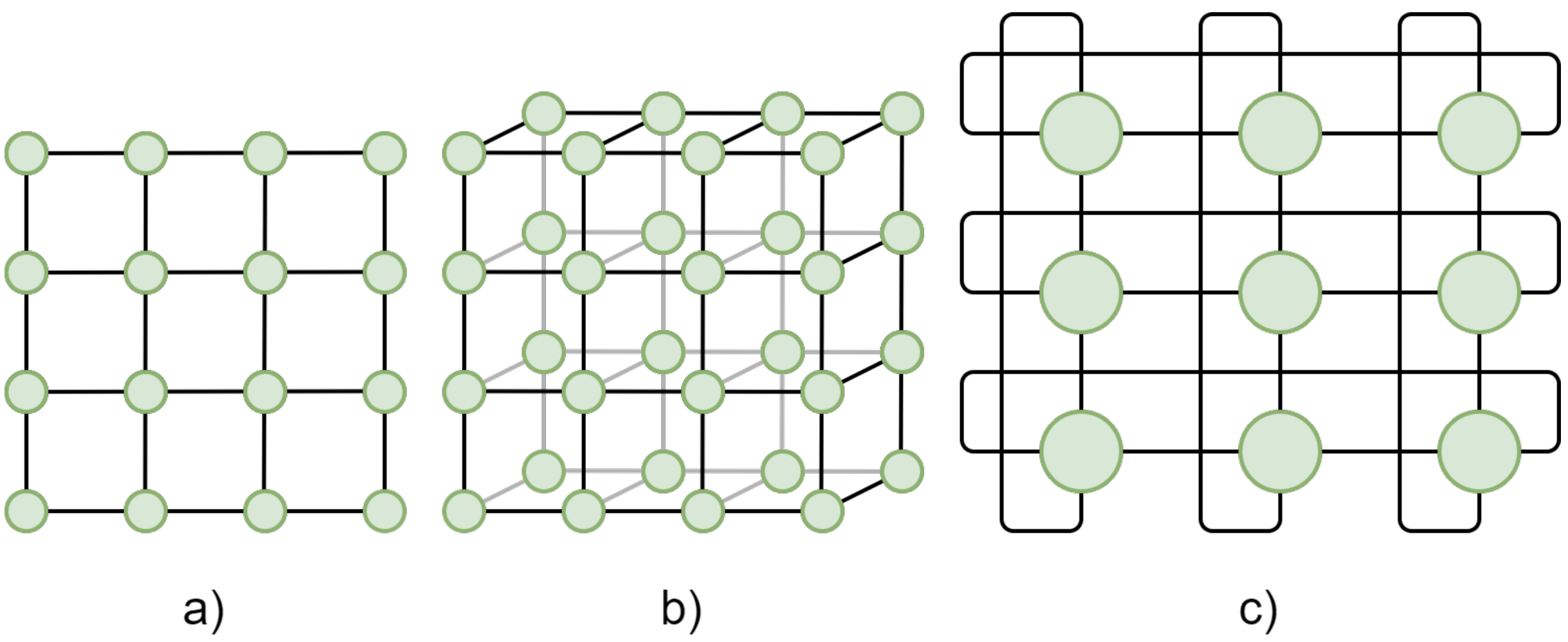
Figure 4: 2D and 3D meshes: a) 2D mesh, b) 3D mesh, c) 2D torus.
Less common HPC topologies include bus, ring, star, hypercube, tree, fully connected, crossbar, and multistage interconnection networks. These topologies are less favorable for general purpose tasks but compute clusters designed for specific use cases may adopt these designs.
HPC networks are also separated into a user-facing front end and a computational back end. The networked compute nodes like those shown in Figure 4 are part of the back end and cannot be accessed directly by the user. Users instead interact with a login node when they conect to an HPC cluster. Here, users can submit jobs to the compute nodes via a workload manager (e.g. sbatch in SLURM).
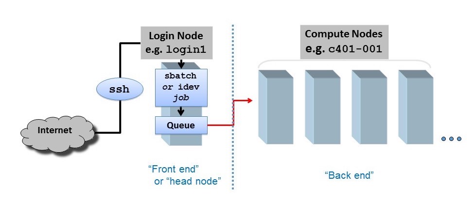
Figure 5: Separation between cluster front end and back end. Credit: https://docs.tacc.utexas.edu/basics/conduct/
Never Run Computations on the Login Node!
When you connect to an HPC cluster, you land on a login node. This shared resource is for compiling resource-light code, managing files, and submitting jobs to the workload manager, but not for heavy computation.
Running an intensive program on the login node will slow it down for everyone, and is a classic mistake for new users.
Submit your job through the workload manager so it runs on compute nodes.
File System
HPC clusters typically provide multiple storage locations, each serving different purposes:
- Home directories: Personal storage for each user, usually with limited capacity. Suitable for scripts, configuration files, and small datasets.
- Scratch: Temporary high-capacity storage for active jobs. Not backed up and typically cleared after job completion. Ideal for:
- Jobs requiring large storage during execution
- Datasets too large for personal storage but not needed permanently
- Jobs needing higher-performance storage than personal directories
- Shared: Storage accessible to multiple users, often for research groups. Commonly used as a shared working directory and generally backed up regularly.
Other types of storage
Large HPC facilities may have a more complex storage organization. For example, there may exist project and archive storages, dedicated to storing large volumes of data that are not accessed often and can tolerate large lags of access time. One of the slowest, but also cheapest and most reliable storage types are magnetic tape libraries. They are commonly used for storing archival (processed with obsolete versions of pipelines) data releases of astronomical surveys, and this system is to be implemented for LSST as well. Always refer to the HPC documentation to understand how storage is implemented in this particular facility - see e.g. Iowa State University or Dartmouth HPC documentation.
Key Points
Communication between different computer components, such as memory and arithmetic/logic unit (ALU), and between different nodes (computers) in a cluster, is often the main bottleneck of the system.
Modern supercomputers are usually assembled from the same parts as personal computers, however, the difference is in the numbers of CPUs, GPUs and memory units, and in the way how they are connected to one another.
Data storage organization varies from one HPC facility to another, so it is necessary to consult documentation when starting the work on a new supercomputer or cluster.
Login nodes must not be used for computationally heavy tasks, as it will slow down the work for all users of the cluster.
LSST HPC facilities and opportunities
Overview
Teaching: 10 min
Exercises: 0 minQuestions
Which HPC facilities are available for the members of the LSST community?
Objectives
Learn about the LSST in-kind contributions that provide HPC capabilities.
Understand the reasoning behind choosing one or another HPC facility.
In the astronomical community, we often have local HPC facilities, most commonly institutional clusters, and for the members of large collaborations, there is usually a possibility to get accesss to large national-level supercomputers. Depending on the project you are part of, you can also have access to the funds for cloud-based HPC solutions, e.g. provided by Google or AWS. However, the LSST community as a whole also has in-house computational facilities that may be used for HPC purposes.
LSST In-Kind program is created to account for non-monetary international contributions to the development and operations of LSST. The idea behind this program is that each participating country has a commitment to contribute a certain amount of research and/or software development efforts, hours of observational time at their observatories, or computational and data storage resources, in exchange for the data rights for the LSST Data Releases for a fixed number of researchers from that country. Among the in-kind contributing teams, there are thirteen computational and data storage facilities. Most of them are considered to be Independent Data Access Centers (IDACs), whose main purpose is to store and provide access to the LSST data products; therefore, they do not always have a significant amount of CPUs or GPUs aboard. However, there are several of them which double as computation centers.
The full list of LSST computational and data storage in-kind contributions can be found in this table. Let’s have a look at the few with HPC capabilities.
Poland IDAC
This light IDAC is located in Poznań Supercomputing and Networking Center (PSNC) and implemented as part of a KMD3/PraceLab2 system, that has about 25 PB of storage and ~6k CPU cores on board, with some GPUs also available. For the LSST users, about 470 CPU cores and about 5 PB of storage will be available. This IDAC is going to store Data Release tables and possibly deep coadd images, and provide access to its databases, CPUs and potentially GPUs with a deployed Rubin Science Platform, multipurpose Jupyter Notebook platform, and SSH connection to Slurm job manager for running code in an HPC mode. The development of this IDAC is in the testing stage. The functionality of this IDAC would be available to all LSST data rights holders. More information can be found here.
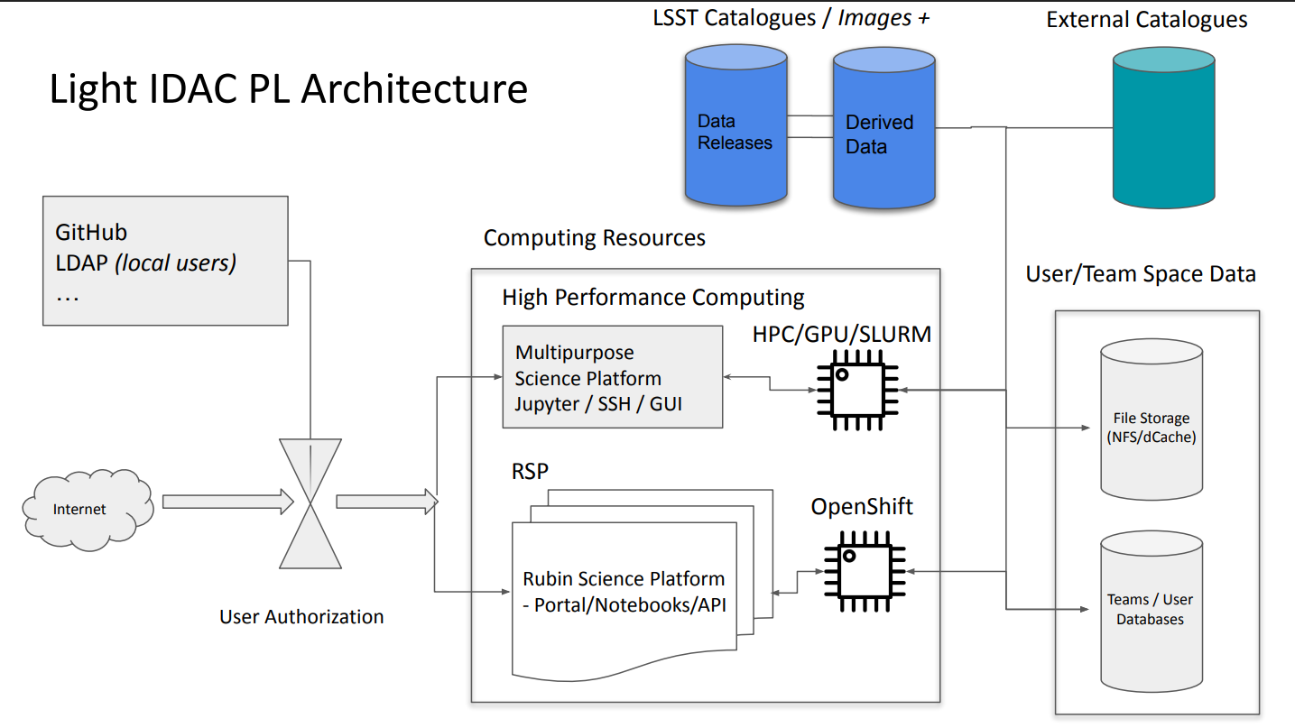
Poland IDAC organization. Credit: Poland IDAC RCW presentation
Brazilian IDAC (LineA)
The Brasilian light IDAC will host catalogs obtained from Data Release coadd images together with a number of secondary data products, such as photo-z catalogues, Solar System tables, catalogues for galactic science, etc. It is a branch of a multi-purpose astronomical platform LineA that already hosts datasets from SDSS, MaNGA, and DES, and provides access to SQL query instruments, Aladin Sky Viewer, Occultation Prediction database, Jupyter Notebooks running on Kubernetes with up to 4 CPU codes and 16 Gb RAM per session, and, upon approval, Jupyter Notebooks running in an HPC mode.
The IDAC will have about 1 PB of user-available storage system and 500 CPU cores. Currently, the system is in beta-testing, but it can be already used by anyone with RSP credentials.
Canadian IDAC
The Canadian IDAC runs on top of the Canadian Astronomy Data Centre (CADC), which hosts data from multiple large-scale surveys, including JWST, HST, Gemini and CFHT. It is available to both Canadian and international users, which, in the case of LSST, means anyone with data rights. By the time of DR1, this IDAC is expected to have 3000 CPUs and 2 PB of long-term user storage dedicated specifically to LSST needs, however, this IDAC uses Jupyter Hub/Jupyter in containers approach, and the maximum amount of resources allocated to one session is up to 16 CPUs and 192 GB of RAM. A batch processing system for jobs is currently being tested, which allows access to larger resources. The most relevant information on this IDAC can be found in the RCW presentation.
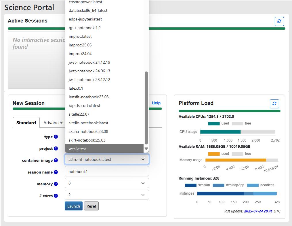
CANFAR service of the Canadian IDAC allows you to run notebooks with a project-specific environment. Credit: Canadian IDAC RCW presentation
Argentina IDAC
Argentina IDAC is envisioned to be an LSST data access point primarily for the Argentinian scientists, however, access can be granted to international collaborators upon agreement. It will carry 1024 CPU cores and 8 GPU Nvidia RTX 6000 Pro Blackwell GPUs, with 3.0 TB RAM and 0.75PB of long-term storage, and is currently being assembled with the planned start of operations in early 2026. The IDAC will host catalogues from the LSST Data Releases, with tentative plans to add object cutouts in the future. The job management will be done with Slurm.
UK Data Facility
The UK Data Facility is, at the moment, the only IDAC that plans to host full LSST Data Releases, including epoch images, together with some user-generated data products. This IDAC does not provide HPC features out of the box - the interface is going to be very similar to the RSP, with Jupyter Notebooks having up to 4 CPU and 16 GB RAM allocated per user. However, batch analysis or ML capabilities from other UK-based facilities may be provided for certain projects. Currently, the IDAC is in preview mode, with the start of operations planned in the next few months.
Croatian SPC (Scientific Processing Center) Bura
One of the Croatian in-kind contributions is computing time on the supercomputer Bura, which we will use during this workshop. Unlike the previous projects, this facility’s primary function isn’t data access, but running HPC calculations. This facility has about 7k CPU nodes with about 95 TB of cluster storage space, together with four GPU nodes. We will talk more about Bura in the next episodes.
Which facility is the right choice for me?
It may seem logical to go for the largest supercomputer available to you, when you need to run some massive computations, however, in practice, there is a number of aspects to consider.
1) Do you need some specific datasets? While obtaining more computational power is relatively simple (to a certain limit), data transfer is still one of the biggest bottlenecks. Transferring many terabytes of data is often problematic, even for large-scale facilities. If you need to perform data analysis on the whole LSST Data Release, especially if you are working with epoch observations, your choice of HPC is severely limited to a few IDACs that store these datasets. The same problem occurs if you need to crossmatch several large datasets.
2) Can your algorithm be implemented on GPUs? If so, is the speed-up crucial? Currently, only a few LSST facilities promise access to GPU computation time, however, institutional clusters are often more advanced in this regard, thanks to the need to serve multiple scientific groups with varying interests. If you are running a Machine Learning algorithm, IDACs are usually not the best choice.
3) Do you use Python, C, or some specific code, e.g. GADGET? Installing software packages on HPCs is less straightforward than it is on a personal computer (and even that is rarely as straightforward as we’d like). Before committing to an HPC facility, write a lightweight testing script that will check that all dependencies needed for your project work properly.
Key Points
Most of the LSST in-kind contributions are IDACs, whose primary function is to provide access to the data products, not run HPC.
Several of the IDACs are based on the already existing computational facilities that do have multiple CPU cores and occasionally GPUs, which may be accessible to the LSST data right holders.
The choice of an HPC facility for your project depends on which datasets you need, whether you can benefit from utilising GPUs, and whether the facility has or allows an easy installation of the necessary dependencies.
Bura access
Overview
Teaching: 20 min
Exercises: 5 minQuestions
How to access the Bura High Performance Computing Cluster
Objectives
Log onto the Bura cluster
Gain familiarity with Bura’s computing resources and capabilities
Intro
Bura is a supercomputer at the Center for Advanced Computing and Modelling (CNRM), University of Rijeka, Croatia. Access to this cluster is available to the Rubin Data Rights community through the LSST International In Kind Program. The goal of this episode is to describe Bura’s architecture and capabilities, and outline the procedure necessary to access the cluster. More detailed information on Bura, including tutorials, can be found here.
The Bura Supercomputer
Bura has a hybrid architecture consisting of three components:
-
Cluster: The system consists of 288 compute nodes, each of which consists of two Xeon E5 processors (with 24 physical cores and 48 threads per node). This gives a total of 6912 processor cores which can support up to 13824 threads. Each node has 64 GB of memory and 320 GB of Solid State Drive (SSD) disk space . In total, the nodes have 18 TB of memory and 95 TB of disk space.
-
GPGPU (General-purpose computing on Graphical Processing Units): This component consists of four nodes, two comprising Xeon E5 processors (each with 8 cores/node) and two based on NVIDIA Tesla K40 general purpose GPUs. 64 GB of RAM is available, with 320 GB of SSD disk space.
-
SMP (Symmetric Multiprocessing): The third component is a multiprocessor system with a large amount of shared memory. The SMP component consists of 16 Xeon E7-8867 processors giving a total of 256 physical cores per node. These have 6 TB of memory and 245 TB of local storage. Two SMP nodes are available.
In addition to the computing nodes, Bura provides some large data storage areas, both of which are accessible from all three components. The first is a 13 TB /home area, and the second is an 868 TB /scatch space. The latter is supported by a Lustre Infiniband parallel distributed filesystem.
Computing on Bura
Bura is designed to provide a multi-user, powerful general-purpose computing environment that can be used for a wide range of applications.
It uses the LMOD system to dynamically manage user environmental modules. This is used to manage user environment variables as well as software dependencies such as Python versions.
Users can run computing tasks on Bura by submitted jobs to its SLURM workload manager. SLURM is an open-source task management system that manages the available computing resources and dynamically schedules the computing tasks submitted by multiple users.
We will cover how to configure and run tasks on Bura in subsequent episodes. Firstly, we need to log into the system.
Accessing Bura

There are two ways to access Bura:
- Using a Virtual Private Network (VPN)
- Through Bura’s web-based portal.
Access through the web browser
You can access Bura simply by opening a new window or tab in your browser and typing Bura’s URL into the address bar:
You should then see the login screen below, where you can enter your user credentials, and click the green “Login” button.

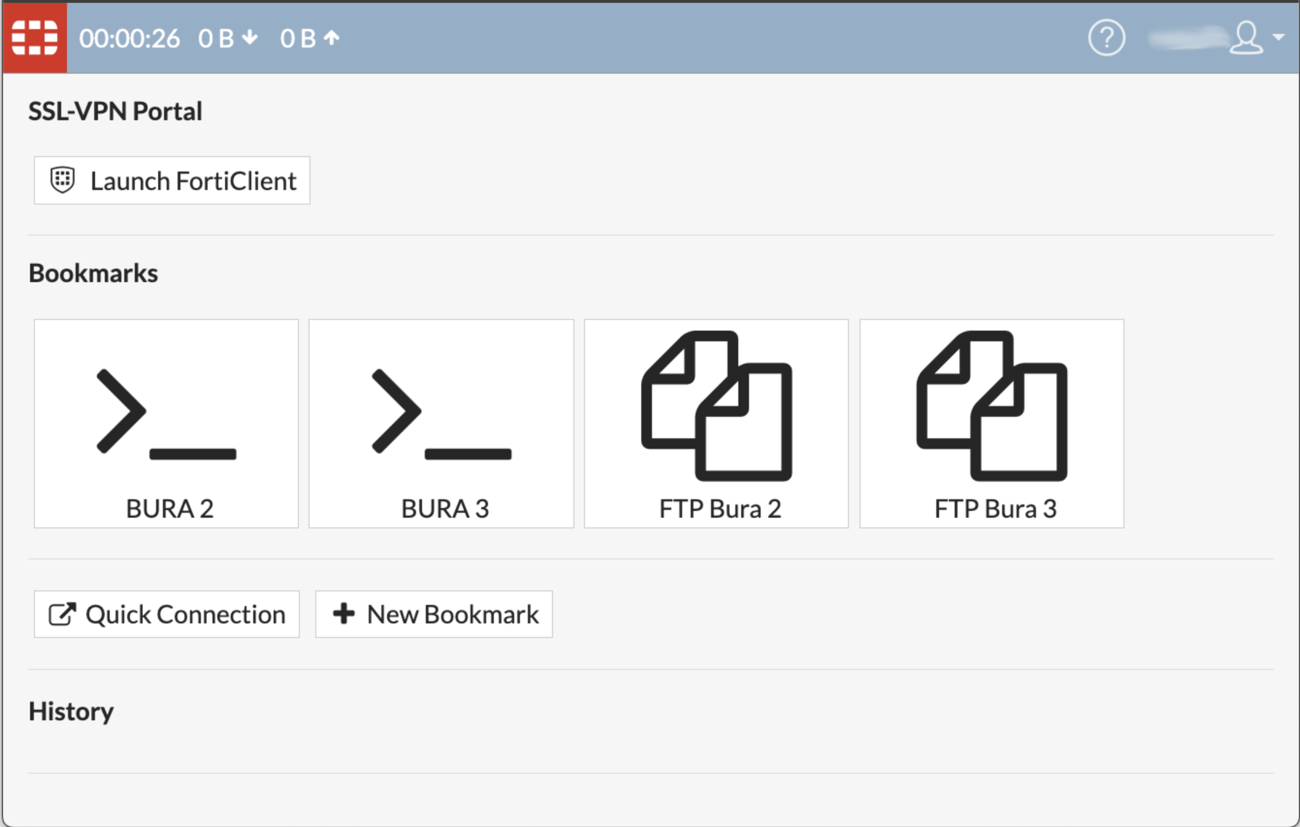
When you have logged in successfully, you will see the following screen:
Please note that there are a few known issues with this method of accessing Bura.
- Some shortcuts don’t work due to the web browser,
- Some lines may be missing. If so, try pressing CTRL-C, and resize the window.
The landing screen offers two options, and you can use either of the Bura2 or Bura3 ports.
FTP File transfer
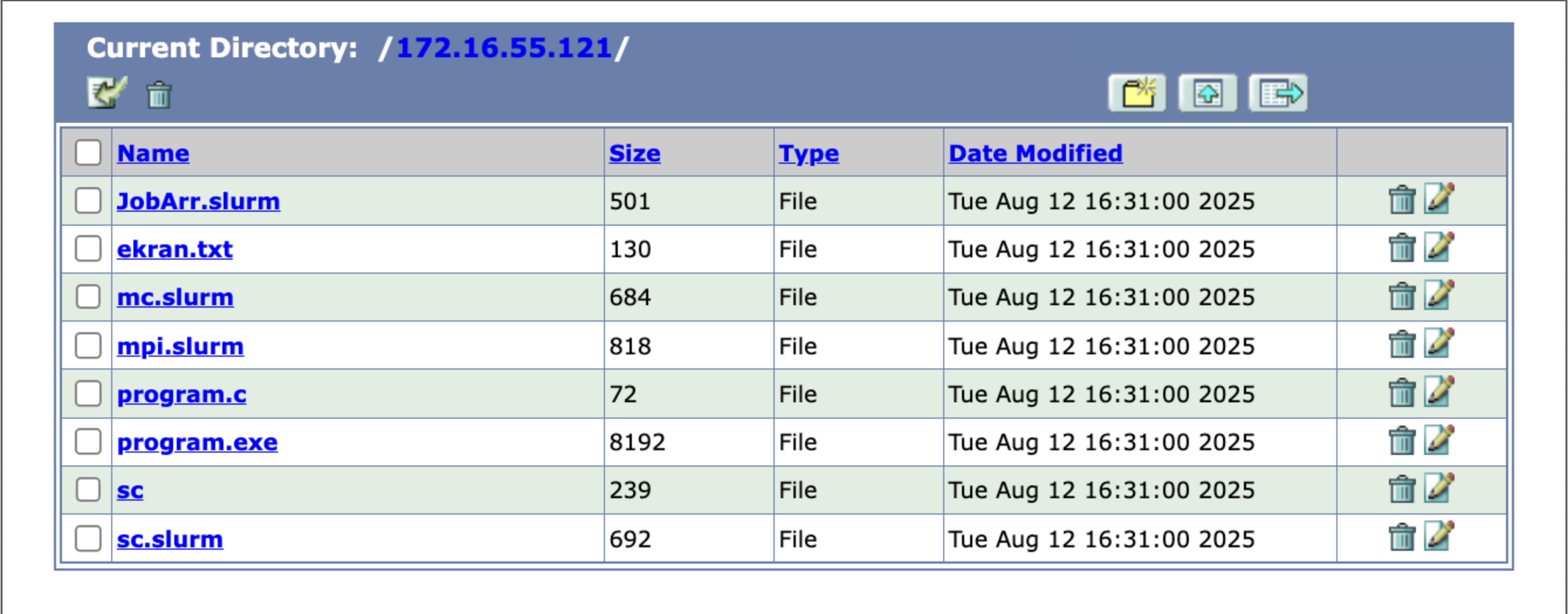
You can transfer files to Bura’s storage areas by clicking on either of the FTP buttons. This will take you to the file system navigator screen, where you can access or add files to your user account’s storage area on Bura.
Starting a terminal session
From the landing page, you can click either of the buttons marked “>_” to start a terminal session which will take you to a Unix-like command prompt.

From here you can start your computing jobs. We will cover how to do that in upcoming episodes.
VPN Access
Alternatively, you can access Bura independently of the web portal by setting up a VPN connection. This requires you to install VPN client software on the machine that you will connect from.
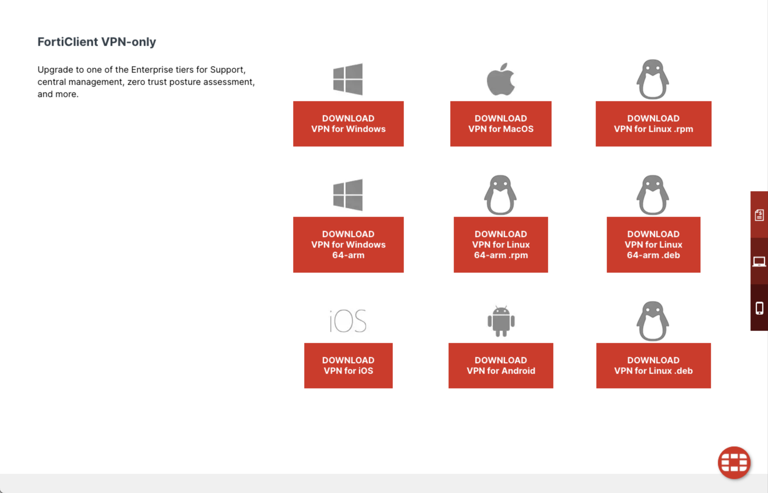
The preferred VPN client is Forticlient, which supports all major operating systems:
- Windows XP, 7, Vista and 10
- Linux Debian, Ubuntu, Centos, Fedora, Redhat and more
- Android
- iOS
- Chromebook
Click here to install Forticlient
Once you have install Forticlient, open the app and use the GUI to add a new connection configuration. The details needed for this configuration were emailed to all workshop participants in advance.
Once the VPN is configured and saved, click the “Connect” slider to open the VPN connection.
Note that it is inadvisable to have multiple VPNs running at the same time, so if the connection is problematic, check to make sure you do not have a different VPN running in the background.
SSH Client
Once you have a secure VPN connection open, it is analogous to creating a secure, private tunnel from your machine to Bura. Traffic, i.e. your commands, can then be sent securely to Bura using the Secure Shell protocol, or SSH.
There are a number of SSH client software packages available for different platforms.
Here we list just a few, but you are welcome to use your preferred client:
- PuTTY (also SuperPutty, PuTTY Tray, KiTTY)
- Bitvise
- MobaXterm (free and pro versions available)
- SmarTTY (free)
- Dameware SSH Client (free and paid versions available)
- mRemoteNG (free)
- Terminals (free)
Whichever client you choose, you should configure the ‘host’ parameter to the IP address of either one of the two Bura login nodes (these were sent to workshop participants by email).
Once you log in with your SSH client you should reach a terminal session and the Bura commandline prompt.
Exercise
Securely log into the Bura cluster through either one of the options described above. Open a terminal session and use the commandline tools described in the previous exercise to list the contents of your home directory and create a new file.
Solution
$ ls
-bash-4.2$ ls
ekran.txt  JobArr.slurm  mc.slurm  mpi.slurm  program.c  program.exe  sc  sc.slurm
$ nano
(Click CTRL-X to exit and save the file with a filename of your choice.)
Key Points
Bura is a powerful supercomputer with CPU, GPGPU and SMP components
Bura can be accessed via a portal through a web-browser, or by installing VPN software and an SSH client
Command line basics
Overview
Teaching: 45 min
Exercises: 15 minQuestions
How can I change directories from the command line?
How can I create directories and files from the command line?
How can I view my identity?
How can I create and move files?
How can I who is doing what on a computer or HPC?
How can I print to the shell?
Objectives
Learn essential shell commands used in data management and processing on a High Performance Computing Environment
Introducing the Shell
The shell or command line is a way to interact with a computer by typing text commands into a terminal or console window. This is in contrast to using a graphical user interface (GUI) with buttons and menus. Although many of the same tasks can be performed with both a shell interface or a GUI interface, the shell gives the most basic and universal access because it does not require any graphics. Whether you’re navigating a High Performance Computing (HPC) repo, inspecting files, or debugging processing failures, these shell commands will be indispensable.
You have already opened a shell to ssh into Bura. Now that your shell is pointing to the Bura file system, we will learn how to navigate it, manipulate files, and interrogate the machine for information about you, the file system, and the tasks it is running.
File Navigation
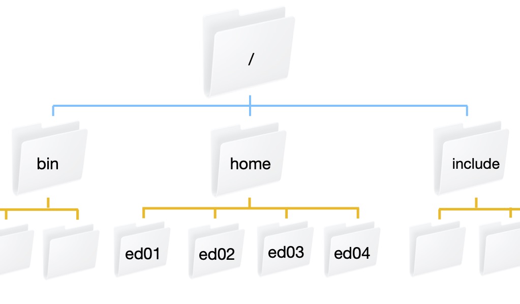
When you view your file system via a graphical interface, you are used to clicking on one folder to look inside and then clicking on another folder inside that one. This folder (or directory) structure is called a directory tree. In the same way that you can click to navigate around your file system, you can type commands into the shell.
Bura is set up with a top level folder or directory /. There are a lot of directories in the the / directory including bin, home, and include. Our individual user directories are contained within the home directory. This figure shows what that directory structure looks like.
What directory am I in?
The pwd command stands for “print working directory”. You can always use this command to ask the shell “where am I?” (you will be surprised how often this comes up).
$ pwd
/home/edu02
What is in my directory?
The ls command is short for listing - this lists all of the files and directories in the directory that you are currently in. This is really helpful if you are looking for something or can’t remember the name of a file or directory.
$ ls
ekran.txt mc.slurm program.c sc JobArr.slurm mpi.slurm program.exe sc.slurm
You can execute this command not only to list all items in your current directory, but in other directories as well. For this, just add the path to the needed directory after the command:
$ ls /home
By default, ls does not show you any directories or files starting with .. These are called hidden files and directories. If you want to see everything, even the hidden files, you can use the -a flag (for all).
$ ls -a
. .. .bash_history ekran.txt JobArr.slurm mc.slurm mpi.slurm program.c program.exe sc sc.slurm
Another useful option is -F flag - this adds symbols to the output to identify different types of entries. For example it will put a / after directories.
Using Multiple Flags
Sometimes you want to use more than one flag for a command (for example maybe you want to use the
-aand-Fflags) to show all hidden files and tell you which ones are directories. If the flag is a single letter then you can string them together likels -aFor if you prefer you can writels -a -F. The order you put the flags in doesn’t matter.
Creating a Directory
When you start a project one of the first things you want to do is set up directories to organize it. For example, you may want a top level directory for the project and then sub-directories for data and code. When you log onto another computer you should not put everything in your home directory. A little organization at the beginning can save you a lot of time later when you try to figure out which files belong to what project. You can create a new directory using the mkdir command (for make directory). Let’s make a directory for the work we do in this course:
$ mkdir hpc_course
Spaces in directory names
You may have noticed that we separate different parts of a command with spaces. The command line uses spaces to parse each part of the command. For this reason, you should not create directories with spaces in them, because if you then try to do something with them from the command line you need to add special characters to group the multiple words together. It is common to use underscores or dashes between words.
Changing Directories
Creating a directory does not move you into the new directory. To change directories you use the cd command. For example:
$ cd hpc_course
To move backwards (or up) a directory (for example to move back to your home directory) use cd ../
Exercise
If you have not already done so, move into your
hpc_coursedirectory. Verify that you are in the correct directory, then create two new directories: code and data. Verify that your directories have been created.Solution
If you haven’t already, move into your hpc_course directory.
$ cd hpc_course

$ pwd
/home/edu02/hpc_course

$ mkdir code
$ mkdir data
$ ls
code  data
Using tab to auto-complete
It can be tiring to type out the name of every file and every directory and it can also be frustrating when you mistype a word. The shell will auto-complete a filename or directory name if you have typed enough of the word to uniquely define it by pressing the tab button. If there is more than one possibility, press the tab button twice to display the different options.
Going backwards
Once you have gone into a directory, how do you get out? ../ is the shells way of saying “go back a directory”. For example, we are currently in the hpc_course directory. If you type cd ../ you will be in your home directory.
$ pwd
 /home/edu02/hpc_course

$ cd ../
$ pwd
/home/edu02

$ ls
ekran.txt  hpc_course  JobArr.slurm  mc.slurm  mpi.slurm  program.c  program.exe  sc  sc.slurm

$ cd hpc_course
Printing to the screen
Sometime you want to write a message to the screen. This can be done with the echo command with the format echo <thing to print>. For example, to print “hello world”:
$ echo "hello world"
hello world
File Manipulation
Shell scripts
Let’s create a simple script that prints “hello world” to the screen. Just like you can write a script in python that executes a series of python commands, you can write a shell script: a text file that contains a series of shell commands. Shell scripting can be very useful in science, including:
- Reproducibility – Shell scripts can be saved and re-executed at a later date. Commands executed in the shell are also saved and can be referred to later.
- Throughput – Many tasks in science are repetitive. For example, if we were conducting a calculation on 100 samples and wanted to do some simple statistics on reads, we could use loops to perform this task on all sets of reads. This is much quicker than using a GUI.
- Integration – Shell scripting allows you to integrate several programs into workflows.
- Efficiency – GUIs can be resource-intensive. Using the shell frees resources that would otherwise be used for the GUI.
Shell scripts are text files that contain shell commands. Our first shell script will print “hello world” to the screen, wait 2 seconds and then exit. We will use the text editor nano. The great thing about nano is that it tells you how to save and exit in the screen, it is also ideal for ssh as it opens directly in the shell window you are using. Here are the most commonly used nano commands:
Ctrl + O— SaveCtrl + X— ExitCtrl + K— Cut lineCtrl + U— Paste line
$ nano shell_example.sh
hello world
In the window that pops up, let’s type echo "hello world" and save and exit. To run your shell script, type:
$ source shell_example.sh
hello world
Pausing for a minute
Sometimes you want your shell script to wait for a little while for a process to finish before it continues with the rest of the commands. The sleep command suspends execution for a specified number of seconds. For example, if you wanted to pause for 5 seconds, you can type:
$ sleep 5
This will wait 5 seconds and then return your cursor to the command line.
Exercise
Use nano to edit your shell_example.sh file to sleep for 2 seconds after it prints “hello world”
Solution
$ nano shell_example.sh
add as a new line
sleep 2

Test your new script
$ source shell_example.sh
hello world
Oops - we just create that script in our top level directory and it belongs in our code directory (because it is a piece of code). We can move the file to the code directory with the mv command. The format is mv thing-you-want-to-move where-you-want-to-move-it
$ mv shell_example.sh code
mv can also be used to rename a file, you can think of this as moving it from one file name to another filename. In this case where-you-want-to-move-it is the new name of the file. Let’s rename the file to something more descriptive hello_world.sh. Don’t forget we moved the file to our code directory, so we have to go there first before we can rename it.
$ ls
code  data

$ cd code
$ ls
shell_example.sh

$ mv shell_example.sh hello_world.sh
$ ls
shell_example.sh
Instead of moving or renaming a file, you can create a copy of the file with the cp command. The format is the same as mv
$ cp hello_world.sh hello_world_copy.sh
$ ls
hello_world_copy.sh hello_world.sh
including paths in cp and mv
You do not always have to be in a directory to copy or move a file. If the file you want to move is not in your current directory, you can refer to the file you want to move with both the path from your current directory and the filename. Similarly, where you want to move a file can also include a path. Let’s say I was in my
hpc_coursedirectory and I want to copy myhello_world.shfile tohello_world_3.sh. The format looks like this:$ pwd /home/edu02/hpc_course/code $ cd ../ $ cp code/hello_world.sh code/hello_world_3.sh
deleting files
You may accidentally create file and want to delete it. This can be done with the rm command which stands for remove. Be careful, the rm command permanently deletes a file - this is not like putting it in the trash can or recycle bin where you can recover it. For that reason, we recommend you use the -i flag which double checks with you before it deletes a file. Now we can remove our hello_world_3.sh file.
$ cd code
$ ls
hello_world_copy.sh  hello_world.sh  hello_world_3.sh

$ rm -i hello_world_3.sh
rm: remove regular file ‘hello_world_3.sh’? y

$ ls
hello_world_copy.sh  hello_world.sh
Exercise
Use nano to edit your
hello_world_copy.shfile to print something else. Rename your file to something descriptive of what it prints. Run your new code.Solution
nano hello_world_copy.shChange “hello world” to “hello universe!”, then save and exit.
$ mv hello_world_copy.sh hello_universe.sh
$ ls
hello_universe.sh hello_world.sh$ source hello_universe.sh
File permissions - who owns what?
Different files on different systems belong to different people and you don’t want anyone to be able to do anything to any file. File permissions restrict access to files and directories based on an individual or a defined group. This is like having a locked office door. There are 3 types of permissions: read (r), write (w), and execute (x). Reading a file allows you to look at the file (or directory) but not modify it. Write permissions allow you to modify the file (or directory). Execute allows you to execute a script. There are also 3 sets of permissions to set: permissions for the owner of the file, permissions for the group that the file belongs to, and permissions for everyone else. Let us take a look at the permissions of the files in our directory. To view the current permissions you can type:
$ ls -l
total 8
-rw-rw-r-- 1 edu02 edu02 32 Aug 16 06:31 hello_universe.sh
-rw-rw-r-- 1 edu02 edu02 28 Aug 16 06:25 hello_world.sh
The output has the following format <type><permissions> <link> <owner> <group> <size> <date modified> <name>. The first character is the type - we will skip this and go directly to the 9 characters after that. The first three are the permissions for the owner. They will always be listed in the order read, write, and execute. If the letter is there than that permission is enabled. For instance if the first three characters were rw- then the owner would have permission to read and write a file or directory but not permission to execute it. The next three characters are the groups permissions. Anyone who belongs to the group listed in the fourth column is assigned these permissions. The permissions work the same way as the owner’s permissions. For instance, if the middle three characters are r-x then anyone in the group has permission to view the file and to execute it, but not to modify it. Finally, the last three characters are for everyone else.
What groups do I belong to?
To figure out what groups you are part of (which can be useful to understand if you have permission to do something) you can type
$ groups
edu02
You modify the permissions on a file or directory using the chmod command. You pass to this command whose permissions you want to modify, owner (o), group (g), everyone else (o), or all users (a), what permission you want to modify (r, w, or x) and whether you want to add (+) that permission or remove (-) it. For example, to give everyone else the ability to execute our hello_world.sh script we would type:
$ ls -l hello_world.sh
-rw-rw-r-- 1 edu02 edu02 28 Aug 16 06:25 hello_world.sh

$ chmod o+x hello_world.sh
$ ls -l hello_world.sh
-rw-rw-r-x 1 edu02 edu02 28 Aug 16 06:25 hello_world.sh
Exercise
What are the permissions on the
hello_universe.sh? Who owns the file? What group does it belong to? Modify the permissions to remove the group’s ability to read the file. Double-check that the permissions changed. Then add the permissions back.Solution
$ ls -l hello_universe.sh
-rw-rw-r-- 1 edu02 edu02 32 Aug 16 06:31 hello_universe.sh

$ chmod g-r hello_universe.sh
$ ls -l hello_universe.sh
-rw--w-r-- 1 edu02 edu02 32 Aug 16 06:31 hello_universe.sh

$ chmod g+r hello_universe.sh
$ ls -l hello_universe.sh
-rw-rw-r-- 1 edu02 edu02 32 Aug 16 06:31 hello_universe.sh
Ethical usage of HPCs
Depending on the permissions set, you may see directories belonging to other users, and sometimes access their content. Simultaneously, other users may have access to your files. Keep this in mind when storing non-public data, such as observations and data releases that are still protected by Data Rights agreements, on third-party computational facilities. Similarly, be mindful when browsing the directories open to you of the possibility that some reading and writing permissions might have been set by mistake.
Understanding what is happening on the whole system
Later in this lesson you will learn how to monitor specific tasks that you run on the HPC. Sometimes you want information about the file system or what processes are running outside of the HPC task manager.
When you are working on an HPC you are using a shared resource. It can be helpful to know how much of that resource you are using. You can do this with the du -h <directory> command. The -h makes the output format human readable (e.g. the size is in Kb, Mb, Gb). First, we will look at the size of our home directory.
How much space am I using?
$ du -h /home/edu02
8.0K	/home/edu02/hpc_course/code
0	/home/edu02/hpc_course/data
8.0K	/home/edu02/hpc_course
52K	/home/edu02
Interrupting a command
Help! you forgot to add a directory and now it is printing the size of every file.
ctl+cwill interrupt the command and return your cursor and command line.
What processes are running and how are they using the HPC?
Another really useful command is seeing what processes are running and who is running them. You can do with the top command.
$ top
The important parts of the output are the PID (process id), USER (who is running the process), %CPU (what percentage of the CPU is being used by that process), %MEM (what percentage of the memory is being used by that process), TIME (how long has the process been running), and COMMAND (what is the command that was run). If you are worried something you did is taking too long or the computer is running slower than you expect, running top is a really good way to get an overview of who is doing what on the system. Note that this will continue to run until you tell it to stop. Type q to exit.
Environment variables
Sometimes you have files and/or paths that you want multiple scripts (in different files) to point to. Instead of hard-coding these in every file, you can create an environment variable that each script can look at to get the file or path name. This means that if you decide to change the path or file, you just have to do it in one place instead of multiple places where its easy to miss one. To view an environment variable that has already been created, you can use echo and the environment variable, preceded by the $. Environment variables are conventionally all upper case. For example, one environment variable that is commonly used is the PATH variable. This tells your shell which directories and sub directories to search to find a command you type. Let us look at what is in our PATH variable by default:
$ echo $PATH
/usr/local/bin:/usr/bin:/usr/local/sbin:/usr/sbin:/home/edu02/.local/bin:/home/edu02/bin
To create an environment variable, you use the export keyword with the syntax export ENV_VARIABLE=value:
$ export DATA_DIR=/home/edu02/hpc_workshop/data
$ echo $DATA_DIR
/home/edu02/hpc_workshop/data
This creates the variable for an individual shell window. If you exit that window, the variable disappears. If you want to make a permanent variable, you can copy and paste the entire export command into your .bashrc or .bash_profile file. This is an invisible file that lives in your home directory and is executed every time you open a shell window; since these files are invisible, you need to use
ls with an -a flag to see them, and to edit them, you have to add a dot before the file name, e.g. nano ~/.bashrc.
Does creating a variable create the directory?
No matter whether you defined the variable only for the duration of the terminal session or in your
.bashrcfile, it is only a variable. The directory itself does not exist unless you runmkdircommand. Try executingcd $DATA_DIR- you will get an error, notifying you that this directory does not exist.
Help! I over wrote my PATH variable and now nothing works
The
PATHvariable tells your shell where to find all of its commands. If you overwrite this, a lot of things break. For this reason you usually append or prepend to yourPATHvariable rather than overwriting it entirely. If you overwrite it you can always close the shell window and reopen it. To append a directory to yourPATHvariable use the:betweenPATHand the new directory. For example, to add acodedirectory to the end of our path we can type:$ export PATH=$PATH:/home/edu02/hpc_workshop/codewhere
edu02is replaced with your Bura user name. Even if this directory does not exist (as it is in our case), nothing breaks, however, the shell will search for the available commands in these non-existing directories as well every time you run a command.
Getting files to and from the HPC
HPCs are a great resource for computing - but they are not a long term storage solution. You will want to move the files from the HPC to a file system that you control. You may also want to prototype a script locally and then move it to the HPC and run it. There are three ways you can move files back and forth: scp, rsync, and using GitHub (or other version control).
scp stands for secure copy. The command format is scp <what you want to copy> <where to put it> and these paths are always specified from where you are. Because you will be going from one system to another - one of the locations will include both the address to the system and the path, separated by a colon. For this part, we will exit Bura. Type exit to return to your local shell.
Now we will use scp to copy our hello_world.sh script to our local directory (.). After executing the scp command you will be asked for your password. Use your ssh password.
$ scp edu02@172.16.55.121:/home/edu02/hpc_course/code/hello_world.sh .
 edu02@172.16.55.121's password:
 hello_world.sh                                     100%  130     0.1KB/s   00:01
Another option for moving files is rsync. This actually checks that the file or directory has been updated and only moves new things. The format is the same as scp: rsync <what you want to copy> <where to put it>.
Another option for moving files is the file transfer protocol ftp and secure file transfer protocol or sftp. This allows you to actually log onto the HPC and upload files from your machine or download them from the HPC to your local machine. To use sftp basic syntax is sftp user@address. You will then be promted for your password. Once you are logged in you can interact with the shell with basic commands like ls and cd. To download a file from the HPC to your local computer type get <filename>. To upload a file from your local machine to the HPC, type put <filename>
Finally, if you are using version control to track your development and have a remote server (e.g. GitHub, Bitbucket). Then you can use this to create another copy of your repository on the HPC and transfer files via the remote server.
Exercise
For this workshop, we will use some scripts that we prepared in advance. You can download them here.0 Then use
scporrsyncto move the files you downloaded for this course to Bura.Solution
Let’s say we have the downloaded
ziparchive located in/home/alex/Downloadsfolder. In this case, we need to open a new terminal tab, and wihtout logging to Bura in this tab execute thescpcommand:$ scp Downloads/Workshop_Materials.zip edu02@172.16.55.121:/home/edu02We’ll be prompted to type our password, and once it’s done, we’ll get a message saying that our file is copied:
Workshop_Materials.zip 100% 18KB 1.1MB/s 00:00Next we should switch to the terminal tab in which we are logged into Bura, and unzip this archive:
unzip Workshop_Materials.zipThe output should be similar to this:
Archive:  Workshop_Materials.zip
  creating: Workshop_Materials/
  inflating: Workshop_Materials/cuda_check.py
  inflating: Workshop_Materials/cuda_exercise.slurm
  inflating: Workshop_Materials/cuda_libraries.slurm
...
Run
lscommand to verify that you have the materials where you want them, and you’re ready for the next day episodes!
Other really useful commands that we do not have time to cover
As you start using an HPC, you might want to check out these commands:
- learning about different command:
man- Viewing files:
head,tail,less,cat- Finding things:
grep,find- Changing ownership:
chown- System management:
df,free -m,ps,killSee the Command Line Interface (CLI) in the Extras menu for even more!
Key Points
Shell skills enable efficient navigation and manipulation local and remote file systems
The shell can be used to identify who you are and what you have access to
The shell can be used to determine what is happening on a system and how you are using the system
Bura Setup
Overview
Teaching: 30 min
Exercises: 15 minQuestions
How do I find and use software on a shared supercomputer?
Why can’t I just use
sudo apt-get installlike on my own machine?How do I manage different versions of the same software?
How can I install Python packages for my project without affecting other users?
Objectives
Understand the purpose of environment modules.
Use
modulecommands to find, load, and manage software.Understand the need for Python virtual environments.
Create and activate a Python virtual environment.
Install project-specific packages using
pipand arequirements.txtfile.
After learning the basic commands for navigating the filesystem, it’s time to learn how to actually use the software on a supercomputer like Bura. On your personal computer, you might use a package manager like apt, yum, or Homebrew, often with administrator (sudo) privileges. On a shared system used by hundreds of people, this isn’t possible. Instead, we use a system called environment modules.
What are Environment Modules?
Think of the cluster as a massive workshop with every tool imaginable stored in cabinets. To work on your project, you don’t bring all the tools to your bench at once. You just get the specific ones you need, like a particular screwdriver or a specific wrench.
Environment modules work the same way. They let you “load” and “unload” specific software packages and versions into your current terminal session, setting up the necessary paths and variables so you can use them.
Finding Available Software
To see the list of all available software “cabinets,” you can use the module avail command. This will show you all the modules you can load. The list can be very long!
Compactifying the Process
The output of
module availcan be overwhelming. You can pipe the output tolessto scroll through it (module avail | less) or togrepto search for something specific (module avail | grep python).
$ module avail
A shorter alias for module avail is ml av, which you might find more convenient.
$ ml av
This still gives a very long list. A more targeted way to find software is with module spider. This command helps you search for a specific package. Let’s say we want to find what versions of the Python programming language are available.
$ module spider python
--------------------------------------------------------------------------------------------------------------------------------------------------------------------------------------------------------------------------
  python:
--------------------------------------------------------------------------------------------------------------------------------------------------------------------------------------------------------------------------
    Versions:
       python/2.7.18
       python/3.8.12
       python/3.9.7
       python/3.10.5
       ...

--------------------------------------------------------------------------------------------------------------------------------------------------------------------------------------------------------------------------
  To find other possible module matches, use "module -r spider '.*python.*'"
  To learn more about a specific module, use "module spider mod-name"
--------------------------------------------------------------------------------------------------------------------------------------------------------------------------------------------------------------------------
module spider shows us all the modules with “python” in their name and the versions available for each.
Loading and Managing Modules
Now that we’ve found the software we want, we need to “load” it into our environment. Let’s load Python version 3.10.5. The command for this is module load.
$ module load python/Python-3.10.5
How can we be sure the module is loaded? We can use module list to see all the currently active modules in our session.
$ module list
Currently Loaded Modulefiles:
  1) python/Python-3.10.5
If you want to unload a module, you can use the command module unload
$ module unload python/Python-3.10.5
If you want to start fresh and unload all your currently loaded modules, you can use module purge.
$ module purge
$ module list
No Modulefiles Currently Loaded.
Note
When you load a module, it’s only for your current login session. If you log out of Bura and log back in later, your modules will be gone. You will need to module load them again for your new session.
Python Virtual Environments
We’ve loaded a system-wide version of Python. Great! But what if your project needs a specific version of a package like numpy, and another one of your projects needs a different version? If you install them globally, you’ll have conflicts.
To solve this, we use virtual environments. A virtual environment is a self-contained directory that holds a specific Python interpreter and all the packages you install for a particular project. It’s like giving your project its own private toolbox.
Creating a Virtual Environment Let’s create a virtual environment for our workshop project. First, make sure you have the Python module loaded, as the virtual environment will be based on it.
$ module load python/Python-3.10.5
Now, we can create the environment using Python’s built-in venv module. Let’s call our environment interpython.
$ python -m venv interpython
If you now use ls, you will see a new directory has been created.
$ ls
interpython
Activating and Deactivating the Environment
Just creating the environment isn’t enough; you have to activate it. Activating the environment modifies your shell’s prompt to let you know it’s active and points it to the Python and pip executables inside that specific environment.
$ source interpython/bin/activate
You’ll know it worked because your command prompt will change to show the environment’s name.
(interpython) $
Now, any Python packages you install will go into the interpython directory, leaving the system’s Python installation clean.
To exit the environment, simply use the deactivate command.
(interpython) $ deactivate
$
Exercise: Parallelization Challenge
Use the following steps to practice basic HPC environment and Python virtual environment commands.
Challenge
- Use
module spiderto find the available versions ofcmake.- Create a directory for a new project called
my_test_project.- Move into that directory.
- Create and activate a Python virtual environment inside it named
test_env.- Deactivate the environment.
Solution
$ module spider cmake
$ mkdir my_test_project
$ cd my_test_project
$ python -m venv test_env
$ source test_env/bin/activate
(test_env) $ deactivate
Installing Project Packages with pip
Most Python projects depend on a set of external libraries. The standard way to manage these is with a requirements.txt file and Python’s package installer, pip.
First, let’s create the requirements file. Make sure you are in your project directory (e.g., interpython is visible when you type ls). Use nano to create a file named requirements.txt.
$ nano requirements.txt
Now, copy and paste the following list of packages into the nano editor by pressing Shift + Insert.
contourpy==1.3.2
cycler==0.12.1
fonttools==4.59.0
kiwisolver==1.4.9
llvmlite==0.44.0
matplotlib==3.10.5
mpi4py==4.1.0
numba==0.61.2
numpy==2.2.6
packaging==25.0
pillow==11.3.0
pyparsing==3.2.3
python-dateutil==2.9.0.post0
six==1.17.0
Save the file and exit nano (press Ctrl+X, then Y, then Enter).
Now, to install these packages, first activate your virtual environment.
$ source interpython/bin/activate
With the environment active, you can now use pip to install everything listed in your requirements file. The -r flag tells pip to read from a file.
(interpython) $ pip install -r requirements.txt
pip will connect to the internet, download all the specified packages and their dependencies, and install them into your interpython virtual environment.
Now we will load all the modules we will need to perform exercises in the next section.
Note
One particular thing to note about bura is that you need to load all the necessary modules and activate your virtual environment before running your slurm script.
Since the python module is already loaded and the virtual environment is already activated leading to this stage in the episode, we will now load the remaining modules
$ module load mpi/intel-2021.5
$ module load gcc/gcc-13.2.0
You are now ready to move on to the next section. This setup ensures that your work is self-contained and reproducible.
Key Points
HPC systems use environment modules to manage shared software.
Use
module availandmodule spiderto find software.Use
module loadto add software to your environment andmodule purgeto remove it.Loaded modules are temporary and reset when you log out.
Python virtual environments (
venv) isolate your project’s dependencies.Always activate a virtual environment before installing packages with
pip.
Introduction to Slurm workload manager
Overview
Teaching: 50 min
Exercises: 15 minQuestions
What is Slurm?
How do I run computing tasks using Slurm?
Objectives
Understand the role and purpose of Slurm
Understand how to create and run a computing task using Slurm
Intro
Slurm is an open source, fault-tolerant, and highly scalable cluster management and job scheduling system for large and small Linux clusters. Slurm requires no kernel modifications for its operation and is relatively self-contained. As a cluster workload manager, Slurm has three key functions. First, it allocates exclusive and/or non-exclusive access to resources (compute nodes) to users for some duration of time so they can perform work. Second, it provides a framework for starting, executing, and monitoring work (normally a parallel job) on the set of allocated nodes. Finally, it arbitrates contention for resources by managing a queue of pending work.
MPI (Message Passing Interface)
In order to execute a set of software instructions simultaneously on multiple computing
nodes in parallel, we need to have a way of sending those instructions to the nodes.
There are standard libraries available for this purpose that use a standardized syntax and
are designed for use on parallel computing architectures like Bura. This is known as a
Message Passing Interface or MPI.
We will go into this topic in more detail later on, but for now it suffices to know that there are different “flavors” of MPI available, and how you use each one depends on which type of MPI you are using.
There are three fundamentally different modes of operation used by these various MPI implementations. Here is how they interact with the Slurm system:
- Slurm directly launches the tasks and performs initialization of communications through the PMI2 or PMIx APIs. (Supported by most modern MPI implementations.)
- Slurm creates a resource allocation for the job and then mpirun launches tasks using Slurm’s infrastructure (older versions of OpenMPI).
- Slurm creates a resource allocation for the job and then mpirun launches tasks using some mechanism other than Slurm, such as SSH or RSH. These tasks are initiated outside of Slurm’s monitoring or control.
Architecture
Slurm is a system used to manage and organize work on a cluster — a group of computers working together to perform complex tasks.
At the core of Slurm is a central manager, called slurmctld, which keeps track of available resources (like CPUs and memory) and assigns jobs to the appropriate computers. There can also be a backup manager that takes over if the main one fails.
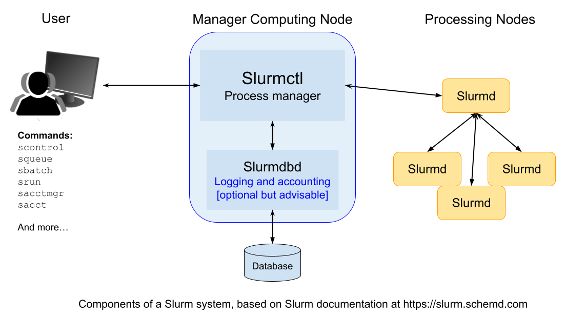
Each computer in the cluster (called a node) runs a program called slurmd. This acts like a remote assistant: it waits for tasks, runs them, sends back results, and then waits for more.
To keep a record of all activity, an optional component called slurmdbd can be used. It stores accounting information — such as who used what resources and when — in a shared database.
Another optional component, slurmrestd, allows users and applications to communicate with Slurm over the web using a REST API.
Users can interact with Slurm from the terminal commandline using several simple commands.
Here are some of the most important ones:
-
srun: starts a job, -
scancel: cancels a running or queued job, -
sinfo: shows the current status of the system, -
squeue: displays information about jobs currently running or waiting, -
sacct: provides detailed reports on finished jobs.
There’s also a graphical interface called sview that visually shows system and job status, including how the nodes are connected.
Administrators can use tools like:
-
scontrol: to monitor or modify how the system is working, -
sacctmgr: to manage users, projects, and resource allocations.
Finally, for developers, Slurm also offers APIs that allow software to interact with the system automatically.
Slurm Commands
Let’s see some of these commands in action. For reference you can find more details about these commands and their options in the SLURM Quick Start Summary (PDF). From the commandline you can also type:
$ man <name of command>
to get more information on all Slurm daemons, commands, and API functions.
The command option –help also provides a brief summary of options. Note that the command options are all case sensitive.
1. View Available Resources
Before we begin a computing task, it is helpful to review what computing resources are
available. The sinfo command reports the state of partitions and nodes managed by Slurm.
# Display the status of partitions (queues) and nodes
sinfo
Expected Output:
PARTITION AVAIL  TIMELIMIT  NODES  STATE NODELIST
debug        up   infinite      2   idle node[01-02]
batch        up   infinite      4   idle node[03-06]
2. Submit a Job Script
Now let’s send a computing task to the Slurm for execution on Bura.
First, create a script file named job.sh. This script provides the Slurm controller with all the information needed to execute the task, including any input data, what commands to execute and where to store any output. The script also controls the number of instances of the job to be run in parallel.
#!/bin/bash
#SBATCH --job-name=test_job       # Name of the job
#SBATCH --output=output.txt       # Save output to this file
#SBATCH --time=00:01:00           # Set max execution time (HH:MM:SS)
#SBATCH --ntasks=1                # Number of tasks to run

hostname                          # Command to execute
We can then submit this job to the Slurm system. Slurm provides a number of ways of doing this.
srun is used to submit a job (an instance of a task) for execution.
$ srun <program>
This command has a wide variety of options to specify resource requirements, which can be configured using optional flags appended to the srun command. Here are a few example of useful flags - see the SLURM Quick Start Summary for a more comprehensive list.
To begin a job at a specific time, e.g. 18:00:00
srun --begin=18:00:00 <program>
To require that a specific number of CPUs be allocated to the task:
srun --cpus-per-task=<Ncpus> <program>
To control the number of instances of the task to be executed:
srun -n<Ntasks> <program>
To assign a maximum time limit after which the job instance should be halted (measured in wall-clock time):
srun --time=<time> <program>
It’s often more convenient to design a job script which can be parallelized over multiple
processes if desired, and submit it for later execution. The sbatch command exists
for this purpose:
sbatch job.sh
Submitted batch job 1234
3. Check the Queue
Having submitted a job, it is very helpful to be able to monitor the status of it. We can do
that using the squeue command - this will show us the status of both running and pending jobs.
squeue
Expected Output:
JOBID PARTITION     NAME     USER ST       TIME  NODES NODELIST(REASON)
1234     batch  test_job   alice  R       0:01      1 node03
4. Cancel a Job
But what do we do if we realise there is a problem with our job after we have submitted it?
We can use the scancel command to cancel a job process. To do so we first need the
jobid assigned to the job once it was submitted. You can find this number from the output
of the squeue command.
E.g., to cancel the job with ID 1234:
scancel 1234
Expected Output:
# No output if successful
5. View Job History
Another useful option is to review a listing of all previous jobs submitted, including those that have been completed (and therefore no longer appear in the output of squeue).
# Show accounting info about completed jobs
sacct
Expected Output:
       JobID    JobName  Partition    State  ExitCode
------------ ---------- ---------- -------- ---------
1234         test_job   batch       COMPLETED      0:0
Deep Dive: sbatch – Submit Jobs to SLURM
Let’s take a closer look at the sbatch command used to submit batch job scripts to
the SLURM job scheduler.
A batch job is a script that specifies what commands to run, what resources to
request, and other scheduling options. When submitted with sbatch, SLURM queues the
job and runs it on an available compute node.
Basic Syntax
sbatch [options] your_job_script.sh

#!/bin/bash
#SBATCH --job-name=my_job          # Name of the job
#SBATCH --output=out.txt           # File to write standard output
#SBATCH --error=err.txt            # File to write standard error
#SBATCH --time=00:10:00            # Time limit (HH:MM:SS)
#SBATCH --ntasks=1                 # Number of tasks
#SBATCH --mem=1G                   # Memory per node
#SBATCH --partition=short          # Partition to submit to

echo "Running on $(hostname)"
sleep 30
| Option | Description |
|---|---|
--job-name=NAME |
Sets the name of the job |
--output=FILE |
Redirects stdout to FILE |
--error=FILE |
Redirects stderr to FILE |
--time=HH:MM:SS |
Sets the time limit for the job |
--ntasks=N |
Number of tasks to run (usually 1 per core unless MPI is used) |
--cpus-per-task=N |
Number of CPU cores per task |
--mem=AMOUNT |
Memory per node (e.g., 4G, 2000M) |
--partition=NAME |
Specifies which partition (queue) to submit to |
--mail-type=ALL |
Sends emails on job start, end, failure, etc. |
--mail-user=EMAIL |
Email address to send notifications to |
--dependency=afterok:ID |
Runs this job only if job with ID completed successfully (afterok) |
Useful Environment Variables
Inside your script, you can use these special variables:
| Variable | Description |
|---|---|
$SLURM_JOB_ID |
The ID of the job |
$SLURM_JOB_NAME |
The name of the job |
$SLURM_SUBMIT_DIR |
The directory from which the job was submitted |
$SLURM_ARRAY_TASK_ID |
The task ID in an array job |
$SLURM_NTASKS |
Total number of tasks requested |
Inline Submission (Without Script)
You can submit commands directly without creating a file:
sbatch --wrap="hostname && sleep 60"
Array Jobs in SLURM
Sometimes you need to run the same job multiple times with slight variations — for example, processing 10 different input files or running a simulation with different parameters.
Instead of writing 10 separate job scripts or submitting the same script 10 times manually, you can use a job array.
SLURM will treat each element in the array as a separate job, but with shared configuration.
Each job will have a unique task ID accessible with the variable $SLURM_ARRAY_TASK_ID.
Example: Simple Job Array
Create a job script named array_job.sh:
#!/bin/bash
#SBATCH --job-name=array_test               # Name of the job
#SBATCH --array=1-10                        # Define array range: 10 jobs with IDs from 1 to 10
#SBATCH --output=logs/job_%A_%a.out         # Output file pattern: %A = job ID, %a = array task ID

echo "This is array task $SLURM_ARRAY_TASK_ID"
What this does:
-
This script will be launched 10 times (one per task).
-
Each task gets a different value of $SLURM_ARRAY_TASK_ID (1 to 10).
-
Each task will write its output to a different file, e.g.:
-
logs/job_1234_1.out
-
logs/job_1234_2.out
-
…
-
logs/job_1234_10.out
-
Monitor Progress
To see the job’s status:
squeue --job 5678
Check Output
Once the job finishes, view the results:
cat out.txt
cat err.txt
Exercise
Create your own Slurm script to run 4 instances of a Python script in parallel, outputting the results to a set of text files.
Solution
Use nano to create a Python script file to be run in parallel (saved to my_python_script.py), e.g.
# Simple example of a python script to be
# run as a Slurm job

# Do some calculation...
result = 100 * 1000

# Output the results to stout.
# This will be captured by the job script and stored
print(result)
Next, create a shell script file (saved to my_job_script.sh) to control the batch process:
#!/bin/bash
#SBATCH --job-name=my_parallel_job
#SBATCH --array=1-4
#SBATCH --output=logs/output_%A_%a.out

python3 my_python_script.py
The use sbatch to submit the job:
$ sbatch my_job_script.sh
Key Points
Slurm is a system for managing computing clusters and scheduling computing jobs
Slurm provides a set of commands which can configure, submit and control jobs on the cluster from the commandline
Jobs can be parallelized using scripts which provide the configuration and commands to be run
Section 2: Running code on Bura
Overview
Teaching: 5 min
Exercises: 0 minQuestions
What are the topics covered in this section?
Objectives
Understand the scope of today’s session.
Activate the virtual environment and load modules needed for the code examples.
In this section, we will do some hands-on exercises to learn what sequential, parallel, and GPU code looks like
in real life, and how to adapt your code when you switch to another code execution mode. We are going to look into why Python relies on other languages, such as C and Cuda,
for massive parallelization, which tools can be used for monitoring the performance of your code and how to use Slurm for running your code across various nodes.
We will use the virtual environment that we created in the previous episodes, so don’t forget to run the commands for activating your environment and loading the modules we’ll use in the code examples:
$ source interpython/bin/activate
$ module load python/Python-3.10.5
$ module load mpi/intel-2021.5
$ module load gcc/gcc-13.2.0
If you missed to create a virtual environment yesterday, you can create it using the following command:
python -m venv interpython
Once you run this, you can then run the commands mentioned above for activating the virtual environment and loading the modules.
Key Points
We will rely on practical exercises to learn what different modes of program execution look like in real life and which tools we can use for performance analysis.
Intro code examples
Overview
Teaching: 15 min
Exercises: 0 minQuestions
What are our options to speed up our code?
Objectives
Understand the main strategies of optimizing code.
Motivation for HPC Coding
Modern computers are fast, however, the volumes of our data and the complexity of our algorithms can easily eat all computational resources and demand more. While most users begin with simple serial code, which runs sequentially on one processor (or rather on a single core), at some point it stops being enough. Maybe we want to model the entire Milky Way using the next big data release from our favorite astronomical survey, or execute high-resolution hydrodynamical simulation, or perform time-critical analysis for follow-up observations, and what took minutes or hours now would take months or years.
So what can we do? There are two main approaches:
-
Approach 1: Make the code faster.
– Use a better algorithm (which is always the preferred way, which, however, may take lots of time and expertise to implement).
– Restructure your code so the CPU works more efficiently, by using vectorization (doing many operations at once inside a single CPU core in a SIMD manner, utilizing internal CPU architecture optimized for this mode of operation) or parallelization (splitting work across multiple cores or machines).
-
Approach 2: Get more computational power.
– Upgrade to a faster processor (with a higher clock speed).
– Use hardware with more processors to implement highly parallelized code. It can be a supercomputer with multiple CPU cores, or a computer with GPUs with thousands of smaller cores.
Before we move on to large-scale supercomputing, let’s first look at a much smaller but very common situation - how a simple piece of code can be written in different ways, and how that affects performance. (Approach 1)
Even if we’re only summing the numbers in a big array, the way we write the code can make a big difference.
A naïve approach (using a for loop) processes one element at a time, while more efficient approaches can take advantage of the CPU’s ability to perform many operations at once.
This idea — doing more work in the same amount of time by restructuring code — is the foundation of high-performance computing.
We’ll start with this simple example to see how writing smarter code (vectorization) can already give us a big speed-up, even before we try parallelization or supercomputers.
Serial vs. Vectorized Code
Let’s look at a simple example: summing the elements of a large array. As mentioned above an obvious way to implement this is by using a for loop. With this implementation, each iteration runs only after the previous one has finished.
# File Name - serial_code.py
# This script demonstrates summing a large NumPy array using a Python loop.
# It highlights the performance cost of looping in Python compared to vectorized operations.

# Import NumPy for numerical array operations and time for measuring execution time
import numpy as np
import time

# Create a NumPy array of 10 million random values between 0 and 1
array = np.random.rand(10**7)

# Record the start time
start = time.time()

# Initialize the total sum
total = 0.0

# Loop over each element in the array and add it to the total
for value in array:
     total += value

# Record the end time
end = time.time()

# Print the final sum and the time taken
print(f"Sum: {total}, Time taken: {end - start:.4f} seconds")
Sum: 4999849.298696889, Time taken: 1.2308 seconds
Depending on your processor, this code may take up to a couple of seconds to execute.
In Python, operations like summation can be written in two different ways: either by looping over elements one at a time, or by using vectorized operations. When we write a loop in Python, the interpreter has to handle each iteration in high-level Python code. This introduces overhead and makes the operation relatively slow.
In contrast, functions like numpy.sum are implemented in optimized C code. C is a low-level, compiled language, which means its instructions run directly on the CPU without the overhead of the Python interpreter. By handing the entire array to numpy.sum, we allow the computation to be carried out in C instead of Python.
Vectorization can be formally defined as the process of expressing operations on entire arrays or vectors of data, rather than performing computations element by element. This allows compilers and libraries to use hardware-level optimizations such as SIMD (Single Instruction, Multiple Data) instructions, which process multiple elements simultaneously.
This approach provides significant speed-ups because it reduces loop overhead and leverages efficient, low-level implementations. As a result, vectorization lets us write clean, high-level Python code while still achieving the efficiency of low-level compiled code.
We will now implement the same code using numpy.sum
# File Name - vector_numpy.py
# This script demonstrates summing a large NumPy array using NumPy's built-in
# vectorized function np.sum, which is much faster than a manual Python loop.

# Import NumPy for numerical array operations and time for measuring execution time
import numpy as np
import time

# Create a NumPy array of 10 million random values between 0 and 1
array = np.random.rand(10**7)

# Record the start time
start = time.time()

# Compute the sum using NumPy's optimized vectorized function
total = np.sum(array)

# Record the end time
end = time.time()

# Print the final sum and the time taken
print(f"Sum: {total}, Time taken: {end - start:.4f} seconds")
Sum: 4999849.29869658, Time taken: 0.0048 seconds
Run this and compare the times. You should see a big difference — vectorization lets you do the same work in far fewer CPU instructions, without paying Python’s loop-by-loop penalty. For such a small task, the loop overhead is actually a big deal.
Reference:
Key Points
Serial code is limited to a single thread of execution, while parallel code uses multiple cores or nodes.
Parallelising our code for CPU
Overview
Teaching: 30 min
Exercises: 20 minQuestions
What is the difference between serial and parallel code?
How do CPU and GPU programs differ?
What tools and programming models are used for HPC development?
Objectives
Understand the structure of CPU and GPU code examples.
Identify differences between serial, multi-threaded, and GPU-accelerated code.
Recognize common programming models like OpenMP, MPI, and CUDA.
Appreciate performance trade-offs and profiling basics.
Parallel CPU Programming
In the previous section, we saw how to make our code faster for sequential jobs. However, there are cases where, no matter how much you optimize, a single process remains a bottleneck. In such cases, we move to parallelization instead of vectorization, especially when computations involve dependencies or irregular structures that cannot be expressed as simple array-wide operations. Some tasks are even embarrassingly parallel meaning they consist of completely independent jobs that you can run side by side, on different CPU cores or separate computers, without any communication.
A perfect example from astronomy is finding stellar variability period from their light curves (measurements of brightness over time). Analyzing one star is quick, but analyzing data from thousands or millions of stars sequentially can take days or weeks. This is where parallel computing becomes essential.
Analyzing Light Curves with Sequential and Parallel Execution
In astronomy, analyzing light curves (the time and brightness data plot of objects in the night sky) is a fundamental task. One common goal is to determine the most likely period of variability, which tells us how often an object repeats its brightness changes.
The Lomb–Scargle Periodogram
To detect periodic signals in light curves, we often use the Lomb–Scargle periodogram.
- A periodogram is a plot of power vs. frequency (or period) that shows how strongly a sinusoidal signal at a given frequency fits the data.
- The Lomb–Scargle method is especially important in astronomy because it works well for unevenly sampled data — a common situation since telescopes can miss nights due to weather, daylight, or scheduling.
- Peaks in the periodogram indicate likely periods of variability, helping us detect signals from variable stars, exoplanets, pulsars, and more.
Sequential vs. Parallel Execution
There are two ways to compute the periodogram for many light curves:
- Sequential execution: analyze one light curve at a time, moving through the dataset in order.
- Parallel execution: split the dataset so that multiple CPU cores each analyze a subset of light curves simultaneously.
Below you can see how the execution time scales up while using the sequential execution vs the parallel execution for detecting the periods of lightcurves using the Lomb–Scargle periodogram

From the plot, we can make the following remarks:
-
For smaller numbers (10, 50, 100, 200, 500, 1000, 5000), the execution time is almost the same for both sequential and parallel runs which are denoted by the blue and the orange lines respectively.
-
This happens because starting and managing parallel jobs has a small extra cost (called overhead).
-
As the number of light curves grows larger (beyond 5000), the benefit of parallelization becomes clear.
-
In the plot:
- Sequential time keeps increasing steadily as the workload grows.
- Parallel time stays much flatter, showing that multiple processes share the work efficiently.
Computational Complexity
The efficiency of both light curve processing and the Lomb–Scargle algorithm depends on their computational complexity.
- For many simple data processing tasks, the time required grows roughly as O(n), meaning if you double the number of data points, the computation takes about twice as long.
- Other algorithms are more expensive, following O(n²) scaling, where doubling the data points makes the computation four times longer.
- The classical Lomb–Scargle periodogram has a complexity of about O(n × m), where n is the number of data points in a light curve and m is the number of trial frequencies tested. In practice, this often behaves closer to O(n²) for dense frequency searches.
- More modern implementations (like the fast Lomb–Scargle) use mathematical tricks to reduce the scaling closer to O(n log n), making them far more efficient for very large datasets.
- Understanding complexity is crucial: it tells us when parallelization will give modest gains (e.g., for O(n) tasks) and when it becomes essential (e.g., for O(n²) or worse).
- Parallelization reduces effective complexity by dividing the work across multiple CPU cores.
- For example, if a task is O(n²) on one processor but can be spread across p processors, the effective runtime becomes closer to O(n² / p).
- While it doesn’t change the theoretical scaling, it reduces the constant factor dramatically, making otherwise infeasible computations practical.
- For small tasks, parallelization does not save time (and may even cost a little extra).
- But as the workload grows, parallelization provides a much more efficient workflow.
Parallel Programming on CPUs
Parallel programming on CPUs is primarily achieved through two widely-used models:
OpenMP (Open Multi-Processing)
OpenMP is used for shared-memory parallelism. It enables multi-threading where each thread has access to the same memory space. It is ideal for multicore processors on a single node.
OpenMP was first introduced in October 1997 as a collaborative effort between hardware vendors, software developers, and academia. The goal was to standardize a simple, portable API for shared-memory parallel programming in C, C++, and Fortran. Over time, OpenMP has evolved to support nested parallelism, Single Instruction Multiple Data (vectorization), and offloading to GPUs, while remaining easy to integrate into existing code through compiler directives.
OpenMP is now maintained by the OpenMP Architecture Review Board, which includes organizations like Arm, AMD, IBM, Intel, Cray, HP, Fujitsu, Nvidia, NEC, Red Hat, Texas Instruments, and Oracle Corporation. OpenMP allows you to parallelize loops in C/C++ or Fortran using compiler directives.
No OpenMP for Python?
While OpenMP is not supported by Python, there are other Python tools that use similar logic. In many cases, when you need to run complex data processing as efficiently as possible, you can use multiprocessing package that allows you to split your dataset into chunks and send them to be processed by different CPU cores.
multiprocessingis a higher-level tool than OpenMP, in the sense that it doesn’t do any kind of optimization on the level of data structures. When performance is really critical, lower-level tools give you more control, but when you want to speed up a processing of a large table from a week to one night,multiprocessingwill do the job.
Terminology
Nested Parallelism
- Nested parallelism occurs when a parallel task itself spawns additional parallel tasks. For example, imagine a program where each thread is responsible for a different data block, and within each block, more threads are launched to handle sub-tasks. This is useful when dealing with hierarchical or recursive algorithms but must be managed carefully to avoid performance penalties due to thread overhead.
Single Instruction, Multiple Data (SIMD) – Vectorization
- SIMD is a form of data-level parallelism where the same instruction operates on multiple data elements simultaneously. For instance, instead of adding two numbers at a time, SIMD allows processors to add pairs of numbers in parallel using wide registers (like 128-bit or 256-bit). Vectorized operations using NumPy or compiler intrinsics take advantage of this under the hood to speed up loops.
Offloading to GPUs
- Offloading refers to transferring compute-intensive tasks from the CPU to the GPU, which is optimized for parallel processing. This is particularly effective for operations that can be executed simultaneously on thousands of threads, like matrix multiplications in deep learning or simulations in scientific computing. Tools like CUDA, OpenCL, or libraries like CuPy and PyTorch help achieve this in Python.
Example: Running a loop in parallel using OpenMP
#include <stdio.h> // For the standard input-output header file (can be thought of as a python library)
#include <omp.h> // For the OpenMP header file (can be thought of as a python library)

int main() {
    int N = 100000;                  // Size of the arrays
    double b[N], c[N], a[N];         // Input and output arrays are defined with fixed lengths

    // Initialize arrays b and c
    for (int i = 0; i < N; i++) {
        b[i] = i * 0.1;
        c[i] = i * 0.2;
    }

    // Parallel loop: compute a[i] = b[i] + c[i]
    #pragma omp parallel for
    for (int i = 0; i < N; i++) {
        a[i] = b[i] + c[i];
    }

    // Print first few values to check
    for (int i = 0; i < 10; i++) {
        printf("a[%d] = %f\n", i, a[i]);
    }

    return 0;
}
Since C programming is not a prerequisite for this workshop, let’s break down the parallel loop code in detail.
Requirements:
- Add
##include <stdio.h>to your code - Add
#include <omp.h>to your code - Compile with
-fopenmpflag
Before we look at the explanation of the C code, we will first look at the Python Equivalent of this code
Python Equivalent of the Code Logic
def add_arrays(b, c):
     """
     Takes two lists `b` and `c`, adds corresponding elements,
     and returns the resulting list `a` where a[i] = b[i] + c[i].
     """
    # Make sure both lists are the same length
    assert len(b) == len(c), "Input arrays must be the same length"

    # Create an output list of the same size
    a = [0.0 for _ in range(len(b))]

    # Loop through and compute a[i] = b[i] + c[i]
    for i in range(len(b)):
        a[i] = b[i] + c[i]

    return a

 # Example usage
 N = 100000
 b = [i * 0.1 for i in range(N)]
 c = [i * 0.2 for i in range(N)]

 a = add_arrays(b, c)

 # Print first few values to verify
 print(a[:10])
In this code snippet, we first define an add_arrays function that sums two lists element-wise,
and then in the main part of the script we define b and c lists and execute add_arrays function. We are treating Python lists as C arrays here,
in the sense that we are doing something unusual for Python when we first define an empty ‘placeholder’ a, and then assign new values to each element of the list in
the for loop. The reason we are doing this and not a.append(b[i] + c[i]) is because we want to preserve each step of the original C code, and in C and C++
there is no possibility to do something like append to the C or C++ plain array
(although there are variable types that allow this behavior, allocating memory in advance is much more efficient).
Explanation of the C code
#include <stdio.h>: Allows use ofprintffor output.#include <omp.h>: Includes the OpenMP API header needed for parallel programming.int N = 100000;: Defines the size of the arrays.double b[N], c[N], a[N];: Declares three arrays of sizeN(two inputs and one output).- The first
forloop initializes arraysbandcwith values (i * 0.1andi * 0.2).#pragma omp parallel for: A compiler directive that tells the compiler to parallelize theforloop that follows.- The second
forloop computes element-wise addition:a[i] = b[i] + c[i].- The final
forloop prints the first 10 elements of the result to verify correctness.How OpenMP Executes This
- OpenMP detects the available CPU cores (e.g., 4 or 8).
- It splits the loop iterations into chunks, assigning each chunk to a different thread.
- Each thread executes its assigned portion of the loop simultaneously (in parallel).
- Once all iterations are done, OpenMP synchronizes the threads automatically.
Output
The output prints the first 10 values of array
a:a[0] = 0.000000 a[1] = 0.300000 a[2] = 0.600000 a[3] = 0.900000 a[4] = 1.200000 a[5] = 1.500000 a[6] = 1.800000 a[7] = 2.100000 a[8] = 2.400000 a[9] = 2.700000
- These values come from
a[i] = b[i] + c[i], whereb[i] = i * 0.1andc[i] = i * 0.2.- Example:
a[1] = (1*0.1) + (1*0.2) = 0.1 + 0.2 = 0.3.
Exercise: Parallelization Challenge
Consider this loop:
#include <stdio.h>

int main() {
    int N = 100000;            // Size of the arrays
    double a[N], b[N];          // Declare input array b and output array a

    // Initialize array b
    for (int i = 0; i < N; i++) {
        b[i] = i * 0.1;
    }

    // Initialize first element of a
    a[0] = b[0];

    // Compute cumulative sum: a[i] = a[i-1] + b[i]
    for (int i = 1; i < N; i++) {
        a[i] = a[i-1] + b[i];
    }

    // Print first few values to verify
    for (int i = 0; i < 10; i++) {
        printf("a[%d] = %f\n", i, a[i]);
    }

    return 0;
}
Can this be parallelized with OpenMP? Why or why not?
Solution
No, this cannot be safely parallelized because each iteration depends on the result of the previous iteration (
a[i-1]).OpenMP requires loop iterations to be independent for parallel execution. Here, since each
a[i]relies ona[i-1], the loop has a sequential dependency, also known as a loop-carried dependency.This prevents naive parallelization with OpenMP’s
#pragma omp parallel for.However, this type of problem can be parallelized using more advanced techniques like a parallel prefix sum (scan) algorithm, which restructures the computation to allow parallel execution in logarithmic steps instead of linear.
MPI (Message Passing Interface)
MPI is used for distributed-memory parallelism. Processes run on separate memory spaces (often on different nodes) and communicate via message passing. It is suitable for large-scale HPC clusters.
MPI emerged earlier, in the early 1990s, as the need for a standardized message-passing interface became clear in the growing field of distributed-memory computing. Before MPI, various parallel systems used their own vendor-specific libraries, making code difficult to port across machines.
In June 1994, the first official MPI standard (MPI-1) was published by the MPI Forum, a collective of academic institutions, government labs, and industry partners. Since then, MPI has become the de facto standard for scalable parallel computing across multiple nodes, and it continues to evolve with versions like MPI-2, MPI-3, MPI-4, and finally MPI-5 released on June 5 2025 which add support for features like parallel I/O and dynamic process management.
MPI allows multiple copies of a program, called processes, to run simultaneously and coordinate work by message passing. Each process has a unique rank, which identifies it within a communicator (a group of processes that can communicate with each other). We will learn about these methods of MPI using the example below which prints the square of the rank of each process.
Example: Implementation of MPI using the mpi4py library in python
# File Name - mpi_example.py
# This script demonstrates a simple MPI program using mpi4py.
# Each process computes the square of its rank and sends the result
# to the root process (rank 0), which gathers and prints all results.

# Import the MPI module from mpi4py
from mpi4py import MPI

# Initialize the default communicator (all processes belong to COMM_WORLD)
comm = MPI.COMM_WORLD

# Get the rank (unique ID) of the current process
rank = comm.Get_rank()

# Get the total number of processes running in this communicator
size = comm.Get_size()

# Each process computes the square of its rank
data = rank ** 2

# Gather all computed data at the root process (rank 0)
all_data = comm.gather(data, root=0)

# Only the root process prints the gathered data
if rank == 0:
    print(all_data)
Let’s see what is happening in this code snippet.
We are using mpi4py to perform a gather operation (collection of results) using the MPI.COMM_WORLD communicator, which shows how multiple programs (called processes) can work together and then share their results.
When you run a program with MPI, you are actually running many copies of the same program at once. Each copy gets a number, called its rank, so if there are 4 processes, their ranks will be 0, 1, 2, and 3.
In the code each process:
- Determines its rank (an integer from 0 to N-1, where N is the number of processes).
- Computes
rank ** 2(the square of its rank). - Uses
comm.gather()to send the result to the root process (rank 0).
Only the root process gathers the data and prints the complete list.
Example Output (4 processes):
- Rank 0 computes
0² = 0 - Rank 1 computes
1² = 1 - Rank 2 computes
2² = 4 - Rank 3 computes
3² = 9The root process (rank 0) gathers all results and prints:[0, 1, 4, 9]
Other ranks do not print anything. This example illustrates point-to-root communication which is useful when one process needs to collect and process results from all workers.
Terminology
Process:
A single copy of your program that runs at the same time as the others.
Analogy: Imagine four students all solving the same type of math problem at once.Rank:
The ID number for each process (starting at 0).
Analogy: Just like students in a classroom might be numbered 0, 1, 2, 3 so the teacher knows who is who.Communicator (
MPI.COMM_WORLD):
The group of all processes that can talk to each other.
Analogy: Think of it as a big group chat that includes everyone.Gather:
A way for many processes to send their results to one chosen process.
Analogy: Everyone puts their homework into the teacher’s basket, and the teacher collects them.Root process:
The process that receives and collects information (by default, rank 0).
Analogy: The teacher who collects the homework and shows the class the results.Point-to-root communication:
A communication pattern where many processes send information to one process.
Analogy: All students talk to the teacher, but not to each other.
Now we will make a slurm script which we learnt about in the slurm section to run the mpi code we just developed using python. Before we develop the actual script let us remind ourselves of the basics of a slurm script
Basics of a Slurm Script Explained
#!/bin/bash
#SBATCH -J jobname                    # Job name
#SBATCH -o outfile.%J                 # Output file
#SBATCH -e errorfile.%J               # Error file
#SBATCH --partition=computes_thin     # Parallel job queue
#SBATCH -N 2                          # Number of compute nodes
#SBATCH -n 24                         # Total number of CPU cores per node
mpirun -np 48 ./mpi_program           # Run with 48 MPI processes (2 nodes × 24 cores)
Script breakdown:
#!/bin/bash: Specifies bash shell for script execution#SBATCH -J jobname: Sets a descriptive job name for easy identification in queue#SBATCH -o outfile.%J: Redirects standard output to a file with job ID#SBATCH -e errorfile.%J: Redirects error messages to separate file#SBATCH --partition=computes_thin: Specifies the queue/partition for sequential jobs#SBATCH -N 2: Requests 2 compute nodes#SBATCH -n 24: Specifies 24 CPU cores per nodempirun -np 48: Launches 48 MPI processes total (2 × 24)
Slurm Script to execute the code
#!/bin/bash
#SBATCH --job-name=mpi_example # Name of the Job
#SBATCH --output=mpi_%j.out # Name of the output file for the Job
#SBATCH --error=mpi_%j.err # Name of the error file for the Job
#SBATCH --partition=computes_thin # Request the appropriate partition for the job
#SBATCH --nodes=2 # Request the appropriate number of computing nodes required for the job
#SBATCH --ntasks=4 # This specifies how many mpi processes will run across the nodes
#SBATCH --time=00:10:00 # This specifies the maximum amount of time that the job will run for
#SBATCH --mem=16G # This specifies the amount of memory which will be allocated for the job

# Load required modules (This is a sanity check in case jobs are not running as required)
module list

# Activate your virtual environment (We have already activated this in terminal so this again a sanity check)
source interpython/bin/activate

# Run the Python mpi script, here the -np flag specifies the number of processes (copies) the mpi program will run
mpirun -np 4 python mpi_example.py
Make sure your virtual environment has mpi4py installed and that your system has access to the OpenMPI runtime via mpirun. Adjust the number of nodes and tasks depending on the cluster policies.
Exercise 1: Gather lists instead of numbers
Modify the code so that instead of collecting
rank ** 2,
each process sends a list of numbers from0torank.Example (4 processes):
- Rank 0 sends
[0]- Rank 1 sends
[0, 1]- Rank 2 sends
[0, 1, 2]- Rank 3 sends
[0, 1, 2, 3]The root process should gather and print:
[[0], [0, 1], [0, 1, 2], [0, 1, 2, 3]]Solution
# File Name - mpi_ex1.py
# This script demonstrates the use of MPI gather with lists using mpi4py.
# Each process creates a list of integers from 0 up to its rank,
# and the root process (rank 0) gathers and prints all the lists.

# Import the MPI module from mpi4py
from mpi4py import MPI

# Initialize the default communicator (all processes belong to COMM_WORLD)
comm = MPI.COMM_WORLD

# Get the rank (unique ID) of the current process
rank = comm.Get_rank()

# Each process creates a list of numbers from 0 to its rank
data = list(range(rank + 1))

# Gather all lists at the root process (rank 0)
all_data = comm.gather(data, root=0)

# Only the root process prints the gathered lists
if rank == 0:
   print(all_data)
Exercise 2: Broadcast after gather
Currently, only the root process (rank 0) collects the data. Modify the code so that after gathering, the root process broadcasts (‘sends’) the complete list back to all processes.
Hint: Use
comm.bcast()aftercomm.gather().
- What happens if each process prints the result after the broadcast?
Solution
# File Name - mpi_ex2.py
# This script demonstrates combining MPI gather and broadcast using mpi4py.
# 1. Each process computes the square of its rank.
# 2. The results are gathered at the root process (rank 0).
# 3. The root process broadcasts the gathered list to all processes.
# 4. Each process prints the final received list.

# Import the MPI module from mpi4py
from mpi4py import MPI

# Initialize the default communicator (all processes belong to COMM_WORLD)
comm = MPI.COMM_WORLD

# Get the rank (unique ID) of the current process
rank = comm.Get_rank()

# Each process computes its rank squared
data = rank ** 2

# Gather all squared values at the root process (rank 0)
gathered = comm.gather(data, root=0)

# Broadcast the gathered list from the root to all processes
result = comm.bcast(gathered, root=0)

# Each process prints the broadcasted result
print(f"Process {rank} received: {result}")
Example output (4 processes):
Process 0 received: [0, 1, 4, 9]
Process 1 received: [0, 1, 4, 9]
Process 2 received: [0, 1, 4, 9]
Process 3 received: [0, 1, 4, 9]
Now all processes have the final list, not just the root.
References:
Key Points
Serial code is limited to a single thread of execution, while parallel code uses multiple cores or nodes.
OpenMP and MPI are popular for parallel CPU programming; CUDA is used for GPU programming.
High-level libraries like Numba and CuPy make GPU acceleration accessible from Python.
Implementing code examples for running on GPU
Overview
Teaching: 30 min
Exercises: 20 minQuestions
How do CPU and GPU programs differ?
What tools and programming models are used for HPC development?
Objectives
Understand the structure of CPU and GPU code examples.
Identify differences between serial, multi-threaded, and GPU-accelerated code.
Recognize common programming models like OpenMP, MPI, and CUDA.
Appreciate performance trade-offs and profiling basics.
GPU Programming
In the previous section, we saw how we can get a significant speedup by parallelizing tasks across a few CPU cores. This is like turning a solo job into a small team effort. But what happens when the calculations within each task are incredibly demanding? For problems involving massive datasets, like complex simulations or training deep learning models, even a dozen CPU cores can struggle to finish in a reasonable time. This is where we need to move from a small team to a massive army of workers: GPUs.
GPU Programming Concepts
GPUs, or Graphics Processing Units, are composed of thousands of lightweight processing cores that are optimized for handling multiple operations simultaneously. This parallel architecture makes them particularly effective for data-parallel problems, where the same operation is performed independently across large datasets such as matrix multiplications, vector operations, or image processing tasks.
Originally designed to accelerate the rendering of complex graphics and visual effects in computer games, GPUs are inherently well-suited for high-throughput computations involving large tensors and multidimensional arrays. Their architecture enables them to perform numerous arithmetic operations in parallel, which has made them increasingly valuable in scientific computing, deep learning, and simulations.
Even without explicit parallel programming, many modern libraries and frameworks (such as TensorFlow, PyTorch, and CuPy) can automatically leverage GPU acceleration to significantly improve performance. However, to fully exploit the computational power of GPUs, especially in high-performance computing (HPC) environments, explicit parallelization is often employed.
CPU vs GPU Architecture
The fundamental difference lies in their design philosophy. CPUs are optimized for low latency on sequential tasks, while GPUs are built for high throughput on parallel tasks.
- CPUs: Few powerful cores, better for sequential tasks.
- GPUs: Many lightweight cores, ideal for parallel workloads.
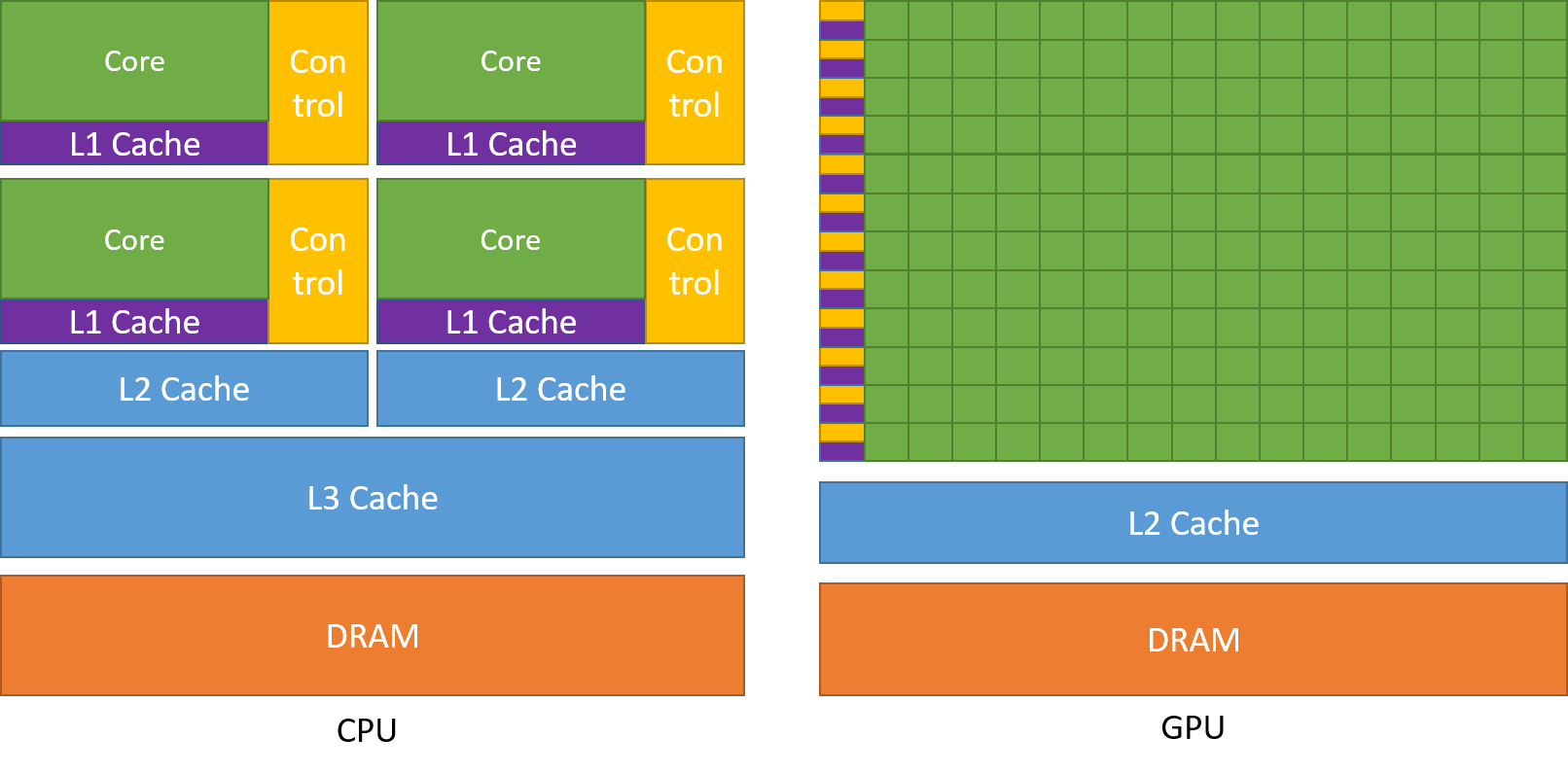
Unlike CPU, that has to handle huge variety of tasks and control data flow in a complicated manner, GPUs dedicate more transistors to data operations. Credit: CUDA C Programming Guide
Comparing CPU and GPU Approaches
| Feature | CPU (OpenMP/MPI) | GPU (CUDA) |
|---|---|---|
| Cores | Few (2–64) | Thousands (1024–10000+) |
| Memory | Shared / distributed | Device-local (needs transfer) |
| Programming | Easier to debug | Requires more setup |
| Performance | Good for logic-heavy tasks | Excellent for large, data-parallel problems |
Introduction to CUDA
In HPC systems, CUDA (Compute Unified Device Architecture), a parallel computing platform and programming model developed by NVIDIA is the most widely used platform for GPU programming. CUDA allows developers to write highly parallel code that runs directly on the GPU, providing fine-grained control over memory usage, thread management, and performance optimization. It allows developers to harness the power of NVIDIA GPUs for general-purpose computing, known as GPGPU (General-Purpose computing on Graphics Processing Units).
In 2006, NVIDIA introduced CUDA, the first platform to provide direct access to the GPU’s virtual instruction set and parallel computational elements. Before CUDA, GPUs were primarily used for rendering graphics, and general-purpose computations required indirect use through graphics APIs like OpenGL or DirectX. CUDA revolutionized scientific computing, deep learning, and high-performance computing (HPC) by enabling massive parallelism and accelerating workloads previously limited to CPUs.
Currently, libraries for writing code in CUDA exist in C, C++, Fortran, and Python. A typical CUDA program runs both on CPU (‘host’) and GPU (‘device’), with CPU responsible for data preparation, memory allocation, and data transfer, and GPU running CUDA kernels, which are essentially functions.
CUDA Hierarchy
There are two aspects to programming for GPU - one is related to the logic of CUDA program, and another is about physical organization of a GPU.
On the logical level, the basic element of CUDA code is a thread. Threads execute the same piece of code (the same kernel), but on different pieces of the data. At every moment, the thread executes only one command. Threads are grouped into blocks, with each block having thousands of threads that have access to the same internal fast shared memory, to which all threads in this block have access, while threads from different blocks have to communicate via global memory. A block can group up to thousands of threads, with a limit determined by the hardware (often it’s 1024 threads). Blocks are then grouped into a grid, which is the highest level of this hierarchy. You can choose the dimensionality of the grid depending on your task - it can be 1D, 2D, or 3D. For example, for image processing, it is often convenient to use 2D grids.
At the level of hardware, each thread corresponds to a core, which is similar to CPU cores, although GPU cores have a simpler design. This is the reason why GPUs can have thousands of cores, while CPUs have only a few dozen. CPU is optimized for the maximum performance of a single-core, sequential code execution, while GPUs are optimized for simultaneous execution of the same simple command on multiple cores. A physical counterpart to the blocks are Streaming Multiprocessors (SM). Each SM contains:
- Many CUDA cores (e.g., 64–128, depending on GPU generation).
- Registers → very fast storage for threads.
- Shared memory → a small, fast memory space for threads in the same block.
-
Schedulers → decide which threads run next. Modern GPUs have tens of SMs, each with dozens of CUDA cores, enabling massive parallelism across the grid.
- Each thread in the grid has a unique ID (
threadIdx) so it knows which piece of data to work on. Depending on the grid dimensionality, the equation for computingthreadIdxwill be different. For example, for a 1D grid, considering that each thread has coordinatesthreadIdx.x,threadIdx.y,threadIdx.z: globalThreadID = blockIdx.x * blockDim.x + threadIdx.x
This formula lets every thread know its global position in the grid.
4. Summary Table
| Level | Unit | Purpose | ID Reference | Hardware Mapping |
|---|---|---|---|---|
| Thread | 1 thread | Smallest unit of computation | threadIdx |
CUDA Core |
| Thread Block | Group of threads | Shares memory, synchronizes threads | blockIdx, threadIdx |
Streaming Multiprocessor (SM) |
| Grid (Kernel) | Block of blocks | Scales to the entire dataset | gridDim, blockDim, threadIdx |
Full GPU |
We can visualise this using the diagrams given below:
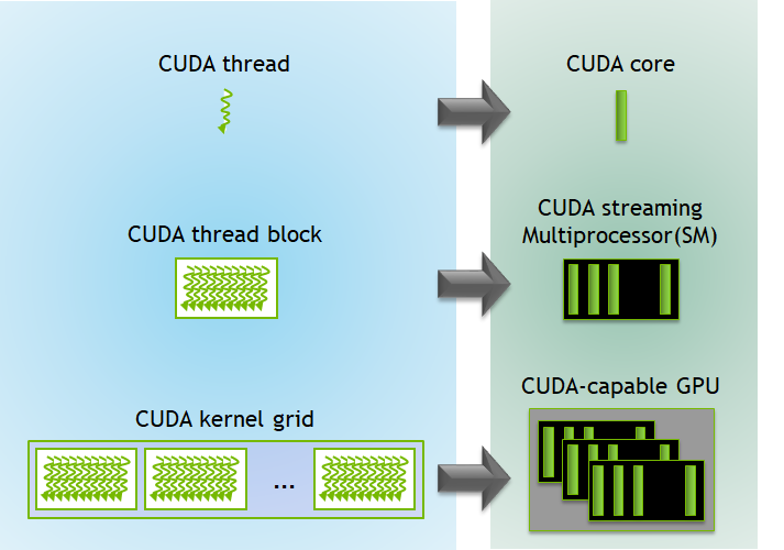
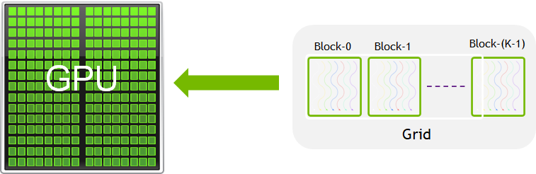
As we already mentioned, a CUDA program includes:
- Host code: Runs on the CPU, manages memory, and launches kernels.
- Device code (kernel): Runs on the GPU.
- Memory management: Host/device memory allocations and transfers.
Therefore, to execute any CUDA program, there are three main steps:
- Copy the input data from host memory to device memory, also known as host-to-device transfer.
- Load the GPU program and execute, caching data on-chip for performance.
- Copy the results from device memory to host memory, also called device-to-host transfer.
CUDA Libraries in Python
When programming GPUs from Python, we can choose between different levels of abstraction. Some libraries hide most of the CUDA details, while others give us fine-grained control. This choice depends on whether you want quick prototyping, large-scale training, or custom GPU kernels.
The high-level libraries handle most CUDA operations automatically. They are easiest to use when your goal is training models or working with arrays without writing GPU kernels.
- PyTorch: Deep learning framework with dynamic computation graphs; move data to GPU with
.to("cuda"). - TensorFlow: Deep learning framework with built-in GPU acceleration; runs on GPU automatically if available.
- JAX: NumPy-like library from Google; uses XLA to JIT-compile code for CPU, GPU (CUDA), and TPU backends.
Mid-Level CUDA Libraries provide a familiar NumPy-like interface but allow more explicit GPU control when needed. An example of such a library is CuPy: Drop-in replacement for NumPy arrays; runs operations on the GPU and also supports writing custom CUDA kernels. Low-level libraries give you the most control. You can write your own GPU kernels and manage device memory directly. In a few minutes we try Numba, which is a JIT compiler for Python; it allows writing custom CUDA kernels using @cuda.jit.
Implementing the libraries to use CUDA
We will now implement vector addition for an input array of one million elements using two approaches: a high-level library (PyTorch) and a low-level library (Numba). These libraries were already installed during the Bura Setup stage of the environment configuration.
Let’s check CUDA availability before running code:
# File Name - cuda_check.py
# This script checks whether CUDA is available using Numba
# and prints the name of the detected GPU if present.

# Import Numba's CUDA module
from numba import cuda

# Check if CUDA-capable GPU is available
if cuda.is_available():
    print("CUDA is available!")

    # Get information about the current GPU device
    print(f"Detected GPU: {cuda.get_current_device().name}")
else:
    print("CUDA is NOT available.")
CUDA is available!
Detected GPU: b'NVIDIA GeForce RTX 3060 Laptop GPU'
Approach 1: Add vectors using the numba Python library
# File Name - numba_cuda.py
# This script demonstrates vector addition on the GPU using Numba's CUDA JIT.
# 1. Define a CUDA kernel for element-wise vector addition.
# 2. Allocate and copy input arrays to the GPU.
# 3. Configure the kernel launch (blocks and threads).
# 4. Run the kernel on the GPU and measure execution time.
# 5. Copy results back to the host and verify correctness.

# Import Numba's CUDA module, NumPy for array operations and time to measure execution time
from numba import cuda
import numpy as np
import time

# @cuda.jit is a decorator provided by Numba.
# It tells Numba to compile the following function (add_vectors) into a CUDA kernel
# that can be executed on the GPU.
# This allows Python code to be transformed into low-level GPU code.
# Therefore @cuda.jit is used to define a CUDA kernel for vector addition
@cuda.jit
def add_vectors(a, b, c):
    # Compute absolute thread index within the entire grid
    i = cuda.grid(1)

    # Perform addition only if within bounds
    if i < a.size:
        c[i] = a[i] + b[i]

# Setup input arrays
N = 1000
a = np.arange(N, dtype=np.float32)
b = np.arange(N, dtype=np.float32)
c = np.zeros_like(a)

# Copy arrays to device
d_a = cuda.to_device(a)
d_b = cuda.to_device(b)
d_c = cuda.device_array_like(a)

# Configure the kernel
threads_per_block = 256
# Typically, GPUs allow up to 1024 threads per block in 1D (depends on GPU architecture).
# Using multiples of 32 is often optimal because of "warps" (groups of 32 threads scheduled together).

blocks_per_grid = (N + threads_per_block - 1) // threads_per_block
# Ensure all elements are covered by rounding up.
# Grid size (total number of threads) = blocks_per_grid * threads_per_block.
# Hardware limitation: Max grid size depends on GPU (often in the range of 2^31-1 for 1D).

# Launch the kernel
start = time.time()
add_vectors[blocks_per_grid, threads_per_block](d_a, d_b, d_c)
cuda.synchronize()  # Wait for GPU to finish
gpu_time = time.time() - start

# Copy result back to host
d_c.copy_to_host(c)

# Verify results
print("First 5 results:", c[:5])
print("Time taken on GPU:", gpu_time, "seconds")
/home/alex/miniconda3/envs/interpython_hpc/lib/python3.13/site-packages/numba/cuda/dispatcher.py:536: NumbaPerformanceWarning: Grid size 4 will likely result in GPU under-utilization due to low occupancy.
  warn(NumbaPerformanceWarning(msg))
First 5 results: [0. 2. 4. 6. 8.]
Time taken on GPU: 0.10699796676635742 seconds
In the Numba example, we see how CUDA works at a low level:
- We first define a GPU kernel using
@cuda.jit. This kernel runs on the GPU and performs vector addition element by element. - The code
@cuda.jitis a decorator. A decorator in Python is essentially a function that modifies or extends the behavior of another function or class without changing its source code. - Basically it passes function
add_vectorsinto the cuda.jit function which turns the python code into low level GPU code. - The function
cuda.grid(1)gives each thread a unique indexi. Each GPU thread computes one element of the result. - We must explicitly copy data from host (CPU) memory to device (GPU) memory with
cuda.to_device. - We also configure how many threads per block and how many blocks per grid to use before launching the kernel.
- Finally, we copy the results back from device to host memory.
This approach is very close to how CUDA is programmed in C/C++. Taking care of threads, blocks, and memory transfers is mandatory when we are doing programming with a low-level tool, such as CUDA.
Python decorators
It is entirely possible that even if you’ve been programming with Python for a long time now, you have never encountered decorators before. They may seem mysterious, however, the idea behind them is quite simple - they are wrapper functions, that accept user-defined function as a parameter. This is possible because in Python, everything is an object, including functions, so you can assign them to a variable, pass as a parameter or return from another function. Common application for decorators is logging or performance measurement, or, as we saw above, a conversion to a format that can be executed on a GPU.
Approach 2: Add vectors using Torch
# File Name - torch_cuda.py
# This script demonstrates performing vector addition on a GPU using PyTorch.
# It highlights how PyTorch can leverage CUDA-enabled GPUs to accelerate
# array operations compared to CPU execution.

# Import PyTorch for GPU-accelerated tensor operations and time for measuring execution time
import torch
import time

# Define the size of the vectors
N = 1_000_000

# Create two input tensors 'a' and 'b' directly on the GPU
# (dtype=float32 for efficiency, device="cuda" ensures they are allocated on GPU)
a = torch.arange(N, dtype=torch.float32, device="cuda")
b = torch.arange(N, dtype=torch.float32, device="cuda")

# Record the start time before performing the vector addition
start = time.time()

# Perform element-wise vector addition on the GPU
c = a + b

# Synchronize with the GPU to ensure that all operations have finished
# (without this, the recorded time may not include the actual GPU computation)
torch.cuda.synchronize()

# Calculate the total elapsed GPU execution time
gpu_time = time.time() - start

# Print the first 5 results of the output vector after moving them back to CPU
# (useful to verify correctness of computation)
print("First 5 results:", c[:5].cpu().numpy())

# Print the total time taken for the GPU computation
print("Time taken on GPU (PyTorch):", gpu_time, "seconds")
First 5 results: [0. 2. 4. 6. 8.]
Time taken on GPU (PyTorch): 0.03913474082946777 seconds
Here, the same operation looks much simpler:
- We create tensors directly on the GPU by specifying
device="cuda". - Adding them with
c = a + bautomatically runs the computation on the GPU. - We call
torch.cuda.synchronize()to make sure the GPU finishes before timing. - If we want to print results, we copy them back to the CPU with
.cpu().numpy().
Here, PyTorch hides all CUDA details. We don’t need to worry about threads, blocks, or explicit memory transfers — the library manages them for us.
Slurm Script to execute the code
The following script can be used to submit a GPU-accelerated Python job (numba_cuda_test.py) using Slurm:
#!/bin/bash
#SBATCH --job-name=cuda_libraries # Name of the Job
#SBATCH --output=cuda_l_%j.out # Name of the output file for the Job
#SBATCH --error=cuda_l_%j.err # Name of the error file for the Job
#SBATCH --partition=gpu # Request the appropriate partition for the job
#SBATCH --nodes=1 # Request the appropriate number of computing nodes required for the job
#SBATCH --cpus-per-task=4 # Request the appropriate number of cpus per computing node required for the job
#SBATCH --mem=16G # This specifies the amount of memory which will be allocated for the job
#SBATCH --gpus-per-node=1 # Request the appropriate number of gpus per computing node required for the job
#SBATCH --time=00:10:00 # This specifies the maximum amount of time that the job will run for

# Load required modules (This is a sanity check in case jobs are not running as required)
module list

# Activate your virtual environment (We have already activated this in terminal so this again a sanity check)
source interpython/bin/activate

# Run the Python example scripts sequentially
python numba_cuda.py
python torch_cuda.py
Exercise: Vector Multiplication on the GPU
In the previous examples, we added two vectors together using Numba and PyTorch.
Now, modify both codes so that they multiply two vectors element by element instead of adding them.
- For Numba: change the CUDA kernel so that each thread multiplies elements instead of adding them.
- For PyTorch: replace the addition operation with multiplication.
Try running your code and compare the results.
Solution
Numba solution:
# File Name - numba_multiplication.py
# This script demonstrates element-wise multiplication of two vectors using Numba with CUDA.
# It highlights how GPU kernels can be written in Python using Numba’s @cuda.jit decorator,
# and how memory needs to be managed explicitly between host (CPU) and device (GPU).

# Import Numba’s CUDA module to write GPU kernels and NumPy for array creation and manipulation
from numba import cuda
import numpy as np

# Define a CUDA kernel function for element-wise vector multiplication
@cuda.jit
def multiply_vectors(a, b, c):
    # Calculate the unique thread index within the grid
    i = cuda.grid(1)

    # Ensure the thread index does not exceed the array size
    if i < a.size:
        c[i] = a[i] * b[i]  # Perform multiplication and store the result

# Define the size of the vectors
N = 10

# Create input arrays on the host (CPU)
a = np.arange(N, dtype=np.float32)   # Vector [0, 1, 2, ..., 9]
b = np.arange(N, dtype=np.float32)   # Vector [0, 1, 2, ..., 9]

# Create an output array initialized with zeros on the host
c = np.zeros_like(a)

# Copy input arrays from host (CPU) to device (GPU)
d_a = cuda.to_device(a)
d_b = cuda.to_device(b)

# Allocate memory on the device for the output array
d_c = cuda.device_array_like(a)

# Define GPU execution configuration
threads_per_block = 256
blocks_per_grid = (N + threads_per_block - 1) // threads_per_block  # Ceiling division

# Launch the kernel with the specified grid and block dimensions
multiply_vectors[blocks_per_grid, threads_per_block](d_a, d_b, d_c)

# Copy the result from device (GPU) back to host (CPU)
d_c.copy_to_host(c)

# Print the result
print("Result (Numba):", c)
/home/alex/miniconda3/envs/interpython_hpc/lib/python3.13/site-packages/numba/cuda/dispatcher.py:536: NumbaPerformanceWarning: Grid size 1 will likely result in GPU under-utilization due to low occupancy. warn(NumbaPerformanceWarning(msg)) Result (Numba): [ 0. 1. 4. 9. 16. 25. 36. 49. 64. 81.]PyTorch solution:
# File Name - torch_multiplication.py
# This script demonstrates element-wise multiplication of two vectors using PyTorch on a GPU.
# It shows how to create tensors directly on the GPU, perform the multiplication operation,
# and then transfer the result back to the CPU for display.

# Import PyTorch for tensor operations
import torch


# Define the size of the vectors
N = 10

# Create a vector of values [0, 1, 2, ..., N-1] stored on the GPU
a = torch.arange(N, dtype=torch.float32, device="cuda")

# Create another vector of values [0, 1, 2, ..., N-1] stored on the GPU
b = torch.arange(N, dtype=torch.float32, device="cuda")

# Perform element-wise multiplication directly on the GPU
c = a * b

# Move the result back to the CPU and convert it to a NumPy array for display
print("Result (PyTorch):", c.cpu().numpy())
Result (PyTorch): [ 0. 1. 4. 9. 16. 25. 36. 49. 64. 81.]Both codes now perform element-wise multiplication instead of addition.
References:
Summary
- Serial code is simple but doesn’t scale well.
- Use OpenMP and MPI for parallelism on CPUs.
- Use CUDA (or high-level wrappers like Numba/CuPy) for GPU programming.
- Always profile your code to understand performance.
- Choose your tool based on problem size, complexity, and hardware.
Key Points
Serial code is limited to a single thread of execution, while parallel code uses multiple cores or nodes.
OpenMP and MPI are popular for parallel CPU programming; CUDA is used for GPU programming.
High-level libraries like Numba and CuPy make GPU acceleration accessible from Python.
Resource requirements
Overview
Teaching: 30 min
Exercises: 10 minQuestions
What is the difference between requesting for CPU and GPU resources using Slurm?
How can I optimize my slurm script to avail the best resources for my specific task?
Objectives
Understand different types of computational workloads and their resource requirements
Write optimized Slurm job scripts for sequential, parallel, and GPU workloads
Monitor and analyze resource utilization
Apply best practices for efficient resource allocation
Understanding Resource Requirements
Different computational tasks have varying resource requirements. Understanding these patterns is crucial for efficient HPC usage.
Types of Workloads
CPU-bound workloads: Tasks that primarily use computational power
- Mathematical calculations, simulations, data processing
- Benefit from more CPU cores and higher clock speeds
Real-world astronomy example:
Calculating theoretical stellar evolution tracks using the MESA code.
Each star’s model requires intense numerical integration of stellar structure equations over millions of time steps, mostly using the CPU.
Memory-bound workloads: Tasks limited by memory access speed
- Large dataset processing, in-memory databases
- Require sufficient RAM and fast memory access
Real-world astronomy example:
Processing full-sky Cosmic Microwave Background (CMB) maps from Planck at high resolution.
The HEALPix maps are large, and operations like spherical harmonic transforms require large amounts of RAM to store intermediate matrices.
I/O-bound workloads: Tasks limited by disk or network operations
- File processing, database queries, data transfer
- Benefit from fast storage and network connections
Real-world astronomy example:
Stacking thousands of raw Rubin Observatory images to improve signal-to-noise ratio for faint galaxy detection.
The bottleneck is reading the large image files from storage and writing processed results back.
GPU-accelerated workloads: Tasks that can utilize parallel processing
- Machine learning, scientific simulations, image processing
- Require appropriate GPU resources and memory
Real-world astronomy example:
Training a convolutional neural network to classify transient events in ZTF light curves.
The matrix multiplications and convolutions benefit greatly from GPU acceleration.
Types of Jobs and Resources
When you run work on an HPC cluster, your job’s type determines how it will be scheduled and what resources it will use. Broadly, jobs fall into three categories:
-
Serial jobs
These use a single CPU core (or sometimes a single thread) to run all calculations. They don’t require communication between multiple processes. They’re ideal for workloads like simple data analysis, single-threaded simulations, or testing code. -
Parallel jobs
These use multiple CPU cores — sometimes across multiple nodes — to run tasks simultaneously. Parallel jobs often use MPI (Message Passing Interface) or OpenMP explained in the previous section to coordinate work. They’re suited for large-scale simulations or computations that can be split into many parts running at once. -
GPU jobs
These use Graphics Processing Units to accelerate certain types of workloads, especially those involving heavy numerical computation like deep learning, image processing, or large matrix operations. GPU jobs often also use CPU cores for parts of the workflow.
Once you know your job type, you can select the correct SLURM partition (queue) and request the right resources:
| Job Type | SLURM Partition | Key SLURM Options | Example Use Case |
|---|---|---|---|
| Serial | computes_thin |
--partition, no MPI |
Single-thread tensor calc |
| Parallel | computes_thin |
-N, -n, mpirun |
MPI simulation |
| GPU | gpu |
--gpus, --cpus-per-task |
Deep learning training |
Choosing the Right Node
- Regular Node: For MPI-based distributed jobs or simple CPU tasks.
- SMP Node (Symmetric Multiprocessing): For jobs needing large shared memory (big matrices, in-memory data) or multi-threaded code (OpenMP, R, Python multiprocessing).
- In an SMP system, multiple CPUs (cores) share the same physical memory and can access it at the same speed. This architecture is ideal when tasks need frequent access to a common memory space without the communication overhead of distributed systems.
- GPU Node: For massively parallel computations on GPUs (e.g., CUDA, TensorFlow, PyTorch).
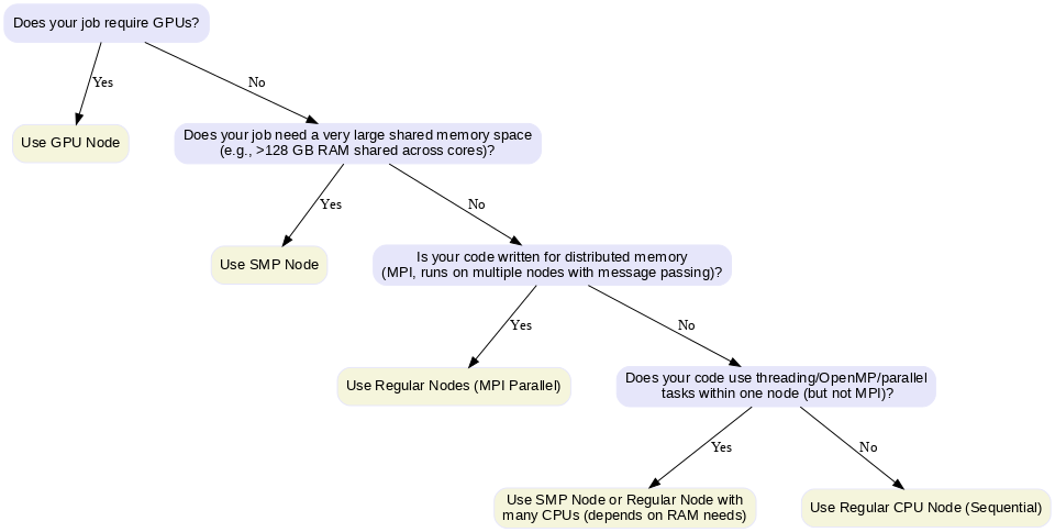
Decision chart for Choosing Nodes
Exercise: Classify the Job Type
Using the decision chart above, classify each of the following HPC tasks into CPU-bound, Memory-bound, I/O-bound, or GPU-accelerated, and suggest the most appropriate node type.
Running a grid of supernova explosion models, varying the star mass, explosion energy, circumstellar density, and radius. Each model runs independently on a separate CPU.
Simulating the galactic stellar population across many spatial grid points for the entire galactic plane. Each grid point is independent; results are aggregated at the end.
- Running the 2D-Hybrid pipeline for periodicity detection on ZTF DR6 quasar light curves:
- Processing objects in batches of 1000 per job.
- Each object is analyzed with wavelet + cross-band methods.
Simulating and fitting microlensing light curves, where each fit is run on a separate CPU, and runtime varies between light curves.
- Distributing difference imaging runs for transient detection using PyTorch, previously run on GPUs, or via MPI/HTCondor.
Discussion:
Are some tasks “mixed-type”? Which resources are more critical for performance? How would you prioritize CPU vs GPU vs memory for these workloads?Solutions
- Grid of supernova explosion models
- Type: CPU-bound (parallel)
- Reason: Each model is independent; heavy numerical computations per model.
- Node type: Regular node (multi-core CPU).
- SLURM options: Use multiple CPUs; each job in the array runs a separate model with
--array=1-100.- Galactic stellar population simulation
- Type: CPU-bound (embarrassingly parallel)
- Reason: Each spatial grid point is independent; computation-heavy but not memory-intensive.
- Node type: Regular node or multi-node if very large. CPUs are sufficient.
- SLURM options: Distribute grid points across CPU cores; use MPI or job arrays with
--ntasks=64.- 2D-Hybrid pipeline for ZTF quasar light curves
- Type: CPU-bound (parallel)
- Reason: Wavelet + cross-band analysis is CPU-only; each batch processed independently.
- Node type: Regular node (multi-core CPU).
- SLURM options: Array jobs with
--cpus-per-taskfor intra-batch parallelization.- Microlensing light curve fitting
- Type: CPU-bound (parallel, varying runtimes)
- Reason: Each light curve fit is independent; some fits take longer than others.
- Node type: Regular node or SMP node if shared memory needed for multithreaded fits.
- SLURM options: Array jobs with
--array=1-999for fitting all light curves.- Difference imaging runs with PyTorch / MPI / HTCondor
- Type: GPU-accelerated (if using PyTorch) or CPU-bound (MPI/HTCondor alternative)
- Reason: GPU use accelerates image subtraction; MPI/HTCondor distributes CPU tasks efficiently.
- Node type: GPU node (for PyTorch) or regular nodes (for MPI/HTCondor).
- SLURM options:
--gpusfor GPU tasks,-N/-nfor MPI tasks.
Key Points
Different computational models (sequential, parallel, GPU) significantly impact runtime and efficiency.
Sequential CPU execution is simple but inefficient for large parameter spaces.
Parallel CPU (e.g., MPI or OpenMP) reduces runtime by distributing tasks but is limited by CPU core counts and communication overhead.
GPU computing can drastically accelerate tasks with massively parallel workloads like grid-based simulations.
Choosing the right computational model depends on the problem structure, resource availability, and cost-efficiency.
Effective Slurm job scripts should match the workload to the hardware: CPUs for serial/parallel, GPUs for highly parallelizable tasks.
Monitoring tools (like
nvidia-smi,seff,top) help validate whether the resource request matches the actual usage.Optimizing resource usage minimizes wait times in shared environments and improves overall throughput.
Resource optimization and monitoring for Serial Jobs
Overview
Teaching: 30 min
Exercises: 10 minQuestions
How do we optimize and monitor resource usage for sequential jobs on an HPC system?
What tools can we use to profile CPU and memory usage for single-core jobs?
What are the best practices and common pitfalls when submitting sequential scripts?
Objectives
Understand how to allocate appropriate resources for sequential (single-core) jobs.
Learn how to monitor CPU and memory usage of sequential jobs on HPC systems.
Use both custom scripts and tools like
htopto profile and optimize job performance.
Example
For understanding how we can utilise different resources available on the HPC for the same computational task, we take the example of a python code which calculates the Gravitational Deflection Angle defined in the following way:
Deflection Angle Formula
For light passing near a massive object, the deflection angle (α) in the weak-field approximation is given by:
α = 4GM / (c²b)
Where:
- G = Gravitational constant (6.67430 × 10⁻¹¹ m³ kg⁻¹ s⁻²)
- M = Mass of the lensing object (in kilograms)
- c = Speed of light (299792458 m/s)
- b = Impact parameter (the closest approach distance of the light ray to the mass, in meters)
Computational Task Description
Compute the deflection angle over a grid of:
- Mass values: From 1 to 1000 solar masses (10³⁰ to 10³³ kg)
- Impact parameters: From 10⁹ to 10¹² meters
Generate a 2D array where each entry corresponds to the deflection angle for a specific pair of mass and impact parameter. Now we will look at how we will implement this for the different resources available on the HPC.
Sequential Job Optimization
Sequential jobs run on a single CPU core and are suitable for tasks that cannot be parallelized. Before that let us again remind ourselves of the structure of a slurm script
Structure of a Slurm Script for a Sequential Job
#!/bin/bash
#SBATCH -J jobname                    # Job name for identification
#SBATCH -o outfile.%J                 # Standard output file (%J = job ID)
#SBATCH -e errorfile.%J               # Standard error file (%J = job ID)
#SBATCH --partition=computes_thin     # Use serial queue for single-core jobs
#SBATCH --nodes=1                     # Serial jobs only require 1 node
#SBATCH --ntasks=1                    # Serial jobs will also require only 1 core
./[programme executable name]         # Execute your program
Example: Gravitational Deflection Angle Sequential CPU
# File Name - example_serial.py
# This script computes the gravitational deflection angle of light around a massive object
# using a nested loop (sequential CPU calculation). It explores a parameter grid of masses
# and impact parameters, saves the computed results to disk, and generates a color plot
# of the deflection angles on a logarithmic scale.

# Import NumPy for numerical array operations, time for measuring execution time, os for appending paths, and matplotlib for plotting the results
import numpy as np
import time
import matplotlib.pyplot as plt
import os
import matplotlib.colors as colors

# Constants
G = 6.67430e-11
c = 299792458
M_sun = 1.98847e30

# Parameter grid
mass_grid = np.linspace(1, 1000, 10000)  # Solar masses
impact_grid = np.linspace(1e9, 1e12, 10000)  # meters

result = np.zeros((len(mass_grid), len(impact_grid)))

# Timing
start = time.time()

# Sequential computation
for i, M in enumerate(mass_grid):
    for j, b in enumerate(impact_grid):
        result[i, j] = (4 * G * M * M_sun) / (c**2 * b)

end = time.time()

print(f"CPU Sequential time: {end - start:.3f} seconds")

result = np.save("result_cpu.npy", result)
mass_grid = np.save("mass_grid_cpu.npy", mass_grid)
impact_grid = np.save("impact_grid_cpu.npy", impact_grid)

# Load data
result = np.load("result_cpu.npy")
mass_grid = np.load("mass_grid_cpu.npy")
impact_grid = np.load("impact_grid_cpu.npy")

# Create meshgrid
M, B = np.meshgrid(mass_grid / 1.989e30, impact_grid / 1e9, indexing='ij')

# Create output directory
os.makedirs("plots", exist_ok=True)

plt.figure(figsize=(8,6))
pcm = plt.pcolormesh(B, M, result,
                      norm=colors.LogNorm(vmin=result[result > 0].min(), vmax=result.max()),
                      shading='auto', cmap='plasma')

plt.colorbar(pcm, label='Deflection Angle (radians, log scale)')
plt.xlabel('Impact Parameter (Gm)')
plt.ylabel('Mass (Solar Masses)')
plt.title('Gravitational Deflection Angle - CPU')

plt.tight_layout()
plt.savefig("plots/deflection_angle_cpu.png", dpi=300)
plt.close()

print("CPU plot saved in 'plots/deflection_angle_cpu.png'")
 CPU Sequential time: 153.965 seconds
 CPU plot saved in 'plots/deflection_angle_cpu.png'
This code simulates gravitational lensing by computing how much light bends when passing near massive objects. It first defines key physical constants, then creates two grids: one for object masses (in solar masses) and one for impact parameters (the distance of closest approach). For every combination of mass and impact parameter, it calculates the deflection angle using the gravitational lensing formula and stores the results in a 2D array. The code measures and prints the runtime to highlight sequential execution speed, saves the computed data for reuse, and finally generates a log-scaled color plot showing how deflection varies with mass and distance, which is stored as an image for visualization.
Job Monitoring and Profiling
We would also want to monitor the resources for the job when we run the job, so we can decide if we allocated the right amount of resources for the job type. For this we will need to create a shell file which logs the CPU and Memory resource usage every five seconds. We can create that file using the code below
#File: monitor_resources.sh
#!/bin/bash
# Monitor CPU% and Memory usage of Python processes for the user (you)
# Saves results in a log file

OUTFILE="resource_usage_${SLURM_JOB_ID}.log"

# Create a header row for the log file
echo "Timestamp | CPU% | Memory(MB)" > "$OUTFILE"

# Repeat until stopped
while true
do
    # ps: shows running processes
    # -u $USER : only show processes owned by you
    # -o %cpu,rss,comm : output CPU%, memory (RSS in KB), and command name
    ps -u $USER -o %cpu,rss,comm \
    | awk '
        $3=="python" {                   # Only lines where command is "python"
            # strftime formats current date/time
            # $1 is CPU%, $2 is memory in KB — divide by 1024 for MB
            print strftime("%Y-%m-%d %H:%M:%S"), "|", $1, "|", $2/1024
        }
    ' >> "$OUTFILE"

    # sleep: pause for 5 seconds before checking again
    sleep 5
done
New Commands and Operators Introduced in this Script
We are using three shell commands and two shell operators:
ps(process status):- The ps command lists processes running on the system. Here, ps -u $USER restricts the list to processes started by the current user. The option -o %cpu,rss,comm customizes the output to show only CPU usage percentage (%cpu), resident memory size in kilobytes (rss), and the command name (comm) like “python”.
awk:- awk is a text processing tool that reads each line of input and allows us to filter or reformat it. In this script, we tell awk to only process lines where the third field (the command name) is “python”. It then prints the current timestamp (strftime), the CPU percentage, and memory converted from kilobytes to megabytes ($2/1024).
sleep:- The sleep command pauses execution for a given number of seconds. Here, sleep 5 makes the script wait 5 seconds before checking the processes again, ensuring we don’t overload the system with constant checks and providing a readable sampling interval.
>(redirect output, overwrite)>creates or overwrites a file with the command’s output.- In this script, it is used once to create the log file and write the header line, replacing any existing file with the same name.
>>(redirect output, append)>>appends output to an existing file instead of overwriting it.- In this script, it is used inside the loop to append each new measurement below the header, so the log grows over time without losing previous entries.
We can now include a command to run this file in the slurm job script that we will use to run the sequential example on BURA.
Sequential Job Script for the Example
#!/bin/bash
#SBATCH --job-name=example_serial # Name of the Job
#SBATCH --output=serial_%j.out # Name of the output file for the Job
#SBATCH --error=serial_%j.err # Name of the error file for the Job
#SBATCH --partition=computes_thin # Request the appropriate partition for the job
#SBATCH --nodes=1 # Request the appropriate number of computing nodes required for the job
#SBATCH --ntasks=1 # This specifies how many processes will run across the nodes
#SBATCH --time=00:10:00 # This specifies the maximum amount of time that the job will run for
#SBATCH --mem=16G # This specifies the amount of memory which will be allocated for the job

# Load required modules (This is a sanity check in case jobs are not running as required)
module list

# Activate your virtual environment (We have already activated this in terminal so this again a sanity check)
source interpython/bin/activate

# Start the resource monitor in the background.
# The "&" symbol is used so the monitor runs simultaneously with the main job instead of blocking it
# The monitor_resources.sh script must be in the same directory as the python file and the slurm script.
bash monitor_resources.sh &

# Run the main sequential job.
python example_serial.py

# Stop the resource monitor after the job finishes.
# "kill %1" is a terminal command which terminates the first background process started in this script.
# Which in our case is monitor_resources.sh.
kill %1

# Print the date and time when the job completed.
echo "Job completed at $(date)"

# Print the name of the log file which was preapared using the resource monitor script
echo "Resource usage saved to resource_usage_${SLURM_JOB_ID}.log"
After we run the script, we can then cat into the resource_usage_${SLURM_JOB_ID}.log file to view the logged CPU and memory usage over time.
Viewing the Results
To quickly view the contents of the log file:
cat resource_usage_${SLURM_JOB_ID}.log
Timestamp           | CPU% | Memory(MB)
2025-08-17 15:32:01 | 95.0 | 1200
2025-08-17 15:32:06 | 99.2 | 1250
2025-08-17 15:32:11 | 100  | 1268
...
Interpreting the Results
CPU%
- For sequential jobs, this should ideally be close to 100%, indicating that the single CPU core is being fully utilized.
- If CPU% is much lower, the program may be waiting on I/O (e.g., reading/writing files) or could benefit from algorithmic optimization.
Memory (MB)
- Shows how much RAM your job is using at each interval.
- Compare the peak memory usage to the memory you requested with
--mem. - If memory usage is consistently much lower than the allocation, you may safely reduce
--memin future runs. - If usage is close to or exceeds your allocation, increase
--memto prevent job crashes.
Quick Reference: Interpreting Resource Usage Patterns
| Pattern | Meaning | Action to Take |
|---|---|---|
| High CPU% (~100%), Low Memory | Code is compute-bound (CPU is the bottleneck, memory not heavily used). | Keep memory request low, focus on algorithmic optimizations or parallelization. |
| Low CPU%, Low Memory | Code is I/O-bound (waiting on file reads/writes or network communication). | Optimize data access, use faster storage, or reduce unnecessary file operations. |
| High CPU%, High Memory | Code is both compute- and memory-intensive. | Ensure enough memory is requested (--mem), and consider algorithm/data structure optimizations. |
| Low CPU%, High Memory | Code is memory-bound (spending more time managing memory than doing compute). | Increase memory allocation, or optimize memory usage in the code (e.g., chunking large arrays). |
| Fluctuating CPU%, Stable Memory | Workload alternates between compute and idle states. | Check for inefficient loops or waiting on external processes; consider restructuring workload. |
| Stable CPU%, Growing Memory | Memory leak (usage increases steadily without bound). | Debug the code, check for objects/arrays not being freed, or optimize memory handling. |
Why This Matters
- Efficient allocation: Avoid over-requesting (slower queue times) or under-requesting (job failures).
- System fairness: Using only what you need helps the scheduler place your jobs more efficiently.
- Debugging: Sudden spikes in memory or drops in CPU can reveal inefficiencies or bugs in your program.
Best Practices and Common Pitfalls for Resource Allocation for Sequential Scripts
Resource Allocation Best Practices
- Request only 1 core
- Sequential jobs run on a single core, so always set
--cpus-per-task=1. - Requesting more cores will not speed up the job and only wastes resources.
- Sequential jobs run on a single core, so always set
- Request memory proportional to workload
- Estimate memory usage (for data arrays, grids, etc.) and add a small safety margin.
- Example: If job needs ~10 GB, request
--mem=12G, not--mem=64G.
- Use appropriate partitions/queues
- Submit sequential jobs to the
serialorthinpartitions if available, instead of compute-intensive queues.
- Submit sequential jobs to the
- Start with test runs
- Run with smaller problem sizes or shorter times first.
- Check logs and resource usage before scaling to full workloads.
- Monitor and refine
- Use tools like
htop,time, or resource monitoring scripts to profile performance. - Adjust memory and runtime allocations based on measured usage.
- Use tools like
Common Pitfalls for Sequential Jobs
Over-requesting resources
   # Bad: Requesting 32 cores for sequential code
   #SBATCH --cpus-per-task=32
   ./sequential_program

   # Good: Match core count to parallelization
   #SBATCH --cpus-per-task=1
   ./sequential_program
Key Points
Sequential jobs only use a single CPU core, so requesting multiple cores wastes resources.
Monitoring resource usage helps match allocation to actual requirements.
htopprovides a quick, interactive way to view CPU and memory consumption.Always start with small test runs and scale resources based on profiling results.
Resource optimization and monitoring for Parallel Jobs
Overview
Teaching: 30 min
Exercises: 10 minQuestions
How do we optimize resource requests for parallel jobs on an HPC system?
What are common pitfalls when requesting CPUs, memory, or nodes?
How can we monitor parallel job performance to adjust allocations?
Objectives
Understand how to request the correct number of nodes, tasks, and memory for MPI jobs.
Learn best practices for parallel job submission to avoid wasted resources.
Use a monitoring script to track CPU and memory usage of parallel jobs in real-time.
Parallel Job Optimization
Parallel jobs can utilize multiple CPU cores across one or more nodes to accelerate computation.
Example: Gravitational Deflection Angle Parallel CPU
# File Name - deflection_angle_mpi.py
# This script computes the gravitational deflection angle of light around a massive object
# using MPI for parallelization across multiple processes. Each MPI rank computes a chunk
# of the mass grid, results are gathered at the root process, and a color plot is generated
# to visualize the deflection angles on a logarithmic scale.

# Import MPI module from mpi4py, NumPy for numerical array operations, time for measuring execution time
# Import os for appending paths, and matplotlib for plotting the results
from mpi4py import MPI
import numpy as np
import time
import os
import matplotlib.pyplot as plt
import matplotlib.colors as colors

# MPI setup
comm = MPI.COMM_WORLD
rank = comm.Get_rank()
size = comm.Get_size()

# Constants
G = 6.67430e-11
c = 299792458
M_sun = 1.98847e30

# Parameter grid (same on all ranks)
mass_grid = np.linspace(1, 1000, 10000)  # Solar masses
impact_grid = np.linspace(1e9, 1e12, 10000)  # meters

# Distribute mass grid among ranks
chunk_size = len(mass_grid) // size # Number of elements assigned to each rank
start_idx = rank * chunk_size # Starting index for this rank
end_idx = (rank + 1) * chunk_size if rank != size - 1 else len(mass_grid) # End index (last rank takes the remainder)

local_mass = mass_grid[start_idx:end_idx]
local_result = np.zeros((len(local_mass), len(impact_grid)))

# Timing
local_start = time.time()

# Compute local chunk
for i, M in enumerate(local_mass):
    for j, b in enumerate(impact_grid):
        local_result[i, j] = (4 * G * M * M_sun) / (c**2 * b)

local_end = time.time()
print(f"Rank {rank} local time: {local_end - local_start:.3f} seconds")

# Gather results
result = None
if rank == 0:
    result = np.zeros((len(mass_grid), len(impact_grid)))

comm.Gather(local_result, result, root=0)

if rank == 0:
    total_time = local_end - local_start
    print(f"MPI total time (wall time): {total_time:.3f} seconds")
    result = np.save("result_mpi.npy", result)
    mass_grid = np.save("mass_grid_mpi.npy", mass_grid)
    impact_grid = np.save("impact_grid_mpi.npy", impact_grid)

# Load data
result = np.load("result_mpi.npy")
mass_grid = np.load("mass_grid_mpi.npy")
impact_grid = np.load("impact_grid_mpi.npy")

# Create meshgrid
M, B = np.meshgrid(mass_grid / 1.989e30, impact_grid / 1e9, indexing='ij')

# Create output directory
os.makedirs("plots", exist_ok=True)

plt.figure(figsize=(8,6))
pcm = plt.pcolormesh(B, M, result,
                      norm=colors.LogNorm(vmin=result[result > 0].min(), vmax=result.max()),
                      shading='auto', cmap='plasma')

plt.colorbar(pcm, label='Deflection Angle (radians, log scale)')
plt.xlabel('Impact Parameter (Gm)')
plt.ylabel('Mass (Solar Masses)')
plt.title('Gravitational Deflection Angle - MPI')

plt.tight_layout()
plt.savefig("plots/deflection_angle_mpi.png", dpi=300)
plt.close()

print("MPI plot saved in 'plots/deflection_angle_mpi.png'")
    Rank 2 local time: 19.160 seconds
    Rank 1 local time: 18.160 seconds
    Rank 3 local time: 17.322 seconds
    Rank 0 local time: 19.576 seconds
    MPI total time (wall time): 19.576 seconds
    MPI plot saved in 'plots/deflection_angle_mpi.png'
We would now again want to monitor the resources, this time for the parallel job, so we can decide if we allocated the right amount of resources for the job. For this we will need to create a shell file which logs the CPU and Memory resource usage of the MPI job every five seconds. We can create that file using the code below
#File: monitor_resources_parallel.sh
#!/bin/bash
# Monitor CPU% and Memory usage of parallel Python (MPI) processes
# Saves results in a log file for later analysis

OUTFILE="resource_usage_${SLURM_JOB_ID}.log"

# Create header
echo "Timestamp | PID | CPU% | Memory(MB) | Command" > "$OUTFILE"

# Repeat until stopped
while true
do
    # List all processes owned by user
    # Filter only python commands (MPI ranks running Python)
    ps -u $USER -o pid,%cpu,rss,comm \
    | awk '
        $4=="python" {
            # rss is memory in KB, convert to MB
            print strftime("%Y-%m-%d %H:%M:%S"), "|", $1, "|", $2, "|", $3/1024, "|", $4
        }
    ' >> "$OUTFILE"

    # Wait 5 seconds before next sample
    sleep 5
done
Explanation of Changes from the Initial Script
The updated monitor_resources_parallel.sh improves the initial monitor_resources.sh while moving to parallel from sequential jobs by adding another column to display the pid or the process id which shows the usage of the CPU% and memory on the different computing nodes requested for our job. This does not show the usage for each indivial copy(rank/number of processes) for the job, but only the total resource usage by the computing nodes.
Parallel Job Script for the Example
#!/bin/bash
#SBATCH --job-name=PCPU # Name of the Job
#SBATCH --output=PCPU_%j.out # Name of the output file for the Job
#SBATCH --error=PCPU_%j.err # Name of the error file for the Job
#SBATCH --partition=computes_thin # Request the appropriate partition for the job
#SBATCH --nodes=2 # Request the appropriate number of computing nodes required for the job
#SBATCH --ntasks=4 # This specifies how many mpi processes will run across the nodes
#SBATCH --time=00:10:00 # This specifies the maximum amount of time that the job will run for
#SBATCH --mem=16G # This specifies the amount of memory which will be allocated for the job

# Load required modules (This is a sanity check in case jobs are not running as required)
module list

# Activate your virtual environment (We have already activated this in terminal so this again a sanity check)
source interpython/bin/activate

# Start the resource monitor in the background.
# The "&" symbol is used so the monitor runs simultaneously with the main job instead of blocking it
# The monitor_resources_parallel.sh script must be in the same directory as the python file and the slurm script.
bash monitor_resources_parallel.sh &

# Save the process ID (PID) of the resource monitor.
# In the serial example, we used "kill %1" to stop the first background job.
# Here we use "$!" to capture the exact PID of the last background process (the monitor), which is safer and more robust.
# Unlike "%1", this works even if there are multiple background processes, since it directly targets the correct one.
MONITOR_PID=$!

echo "Starting MPI job..."

# Run the Python mpi script, here the -np flag specifies the number of processes (copies) the mpi program will run
mpirun -np 4 python example_parallel.py

# Stop the resource monitor once the job is done.
# This ensures the monitor doesn’t keep running after the main program finishes.
kill $MONITOR_PID

# Print the date and time when the job completed.
echo "Job completed at $(date)"

# Print the name of the log file which was preapared using the resource monitor script
echo "Resource usage saved to resource_usage_${SLURM_JOB_ID}.log"
After we run the script, we can then cat into the resource_usage_${SLURM_JOB_ID}.log file to view the logged CPU and memory usage over time.
Viewing the Results
To quickly view the contents of the log file:
cat resource_usage_${SLURM_JOB_ID}.log
Timestamp            | PID   | CPU% | Memory(MB) | Command
2025-08-17 15:01:12  | 12345 | 98.5 | 250.1      | python
2025-08-17 15:01:17  | 12346 | 97.8 | 248.9      | python
Monitoring the parallel script using psutil
A more convenient approach for job monitoring is to use the Python package psutil. It allows us to collect resource usage information from within our script itself along with allowing us to accurately track the CPU% and memory usage for each indivial copy(rank/number of processes) instead of just checking the usage of the computing nodes.
# File Name - deflection_angle_mpi_monitor.py
# This script computes the gravitational deflection angle of light around a massive object
# using MPI for parallelization across multiple processes. Each rank computes a portion
# of the mass grid and the results are gathered at the root process.
# Additionally, each rank launches a background monitoring thread that periodically logs
# CPU and memory usage during execution. The root process generates a heatmap plot of the
# deflection angle results using a logarithmic color scale.

# Import MPI module from mpi4py, NumPy for numerical array operations, time for measuring execution time
# Import os for appending paths, matplotlib for plotting the results, and psutil for resource monitoring
from mpi4py import MPI
import numpy as np
import time
import os
import psutil
import threading
import matplotlib.pyplot as plt
import matplotlib.colors as colors

# MPI setup
comm = MPI.COMM_WORLD
rank = comm.Get_rank()
size = comm.Get_size()

# Constants
G = 6.67430e-11
c = 299792458
M_sun = 1.98847e30

# Monitoring setup
pid = os.getpid()
process = psutil.Process(pid)

def monitor(interval=5):
    """Continuously log CPU and memory usage every `interval` seconds."""
    while True:
        cpu = process.cpu_percent(interval=None)   # CPU usage %
        mem = process.memory_info().rss / (1024*1024)  # Memory in MB
        print(f"[Rank {rank}] CPU%: {cpu:.1f} | Mem: {mem:.2f} MB", flush=True)
        time.sleep(interval)

# Start monitoring thread (all ranks or just rank 0)
t = threading.Thread(target=monitor, daemon=True)
t.start()

# Parameter grid (same on all ranks)
mass_grid = np.linspace(1, 1000, 10000)   # Solar masses
impact_grid = np.linspace(1e9, 1e12, 10000)  # meters

# Divide work among ranks
chunk_size = len(mass_grid) // size
start_idx = rank * chunk_size
end_idx = (rank + 1) * chunk_size if rank != size - 1 else len(mass_grid)

local_mass = mass_grid[start_idx:end_idx]
local_result = np.zeros((len(local_mass), len(impact_grid)))

# Timing + Computation
local_start = time.time()

for i, M in enumerate(local_mass):
    for j, b in enumerate(impact_grid):
        local_result[i, j] = (4 * G * M * M_sun) / (c**2 * b)

local_end = time.time()
print(f"[Rank {rank}] Local compute time: {local_end - local_start:.3f} seconds")

# Gather results
result = None
if rank == 0:
    result = np.zeros((len(mass_grid), len(impact_grid)))

comm.Gather(local_result, result, root=0)

# Post-processing + Plotting
if rank == 0:
    total_time = local_end - local_start
    print(f"[Rank 0] MPI total time (wall time): {total_time:.3f} seconds")

    # Save results
    np.save("result_mpi.npy", result)
    np.save("mass_grid_mpi.npy", mass_grid)
    np.save("impact_grid_mpi.npy", impact_grid)

    # Reload for plotting
    result = np.load("result_mpi.npy")
    mass_grid = np.load("mass_grid_mpi.npy")
    impact_grid = np.load("impact_grid_mpi.npy")

    # Create meshgrid
    M, B = np.meshgrid(mass_grid, impact_grid / 1e9, indexing='ij')

    # Create output directory
    os.makedirs("plots", exist_ok=True)

    # Plot results
    plt.figure(figsize=(8,6))
    pcm = plt.pcolormesh(B, M, result,
                         norm=colors.LogNorm(vmin=result[result > 0].min(), vmax=result.max()),
                         shading='auto', cmap='plasma')

    plt.colorbar(pcm, label='Deflection Angle (radians, log scale)')
    plt.xlabel('Impact Parameter (Gm)')
    plt.ylabel('Mass (Solar Masses)')
    plt.title('Gravitational Deflection Angle - MPI with Monitoring')

    plt.tight_layout()
    plt.savefig("plots/deflection_angle_mpi.png", dpi=300)
    plt.close()

    print("MPI plot saved in 'plots/deflection_angle_mpi.png'")
What Changed in the code
Compared to the earlier version of the MPI script, the scientific workflow (splitting work across ranks, computing deflection angles, gathering results, and plotting) remains the same.
The main change in the final version is the addition of a resource monitoring component:
- psutil integration
- Each MPI rank now imports and uses the
psutillibrary. psutil.Process()gives access to the rank’s own process information (CPU usage, memory usage, etc.).
- Each MPI rank now imports and uses the
- Background monitoring thread
- A lightweight thread is started on each rank.
- This thread runs independently of the computation, waking up every few seconds to record:
- CPU percentage used by that rank.
- Memory usage in MB.
- The results are printed with the rank number (e.g.,
[Rank 2] CPU%: 99.8 | Mem: 350.25 MB).
- Unified output
- Instead of saving to a separate log file (like the shell script), the monitoring results are written directly into the job’s standard output, alongside the scientific results.
- This way, you can see both the computation progress and the resource usage together in real time.
In short, the final script is the original scientific MPI program plus a built-in live performance monitor, achieved by combining psutil (to gather resource stats) with threading (to run the monitor in the background without interrupting the main calculations).
Viewing the Results
To quickly view the contents of the log file:
cat PCPU_${SLURM_JOB_ID}.out
[Rank 1] CPU%: 0.0 | Mem: 219.05 MB
[Rank 0] CPU%: 0.0 | Mem: 230.35 MB
[Rank 2] CPU%: 0.0 | Mem: 230.82 MB
[Rank 3] CPU%: 0.0 | Mem: 227.89 MB
[Rank 1] CPU%: 100.2 | Mem: 272.06 MB
[Rank 0] CPU%: 100.0 | Mem: 279.32 MB
[Rank 2] CPU%: 100.2 | Mem: 283.75 MB
[Rank 3] CPU%: 100.4 | Mem: 280.70 MB
[Rank 1] CPU%: 100.2 | Mem: 328.06 MB
[Rank 0] CPU%: 100.4 | Mem: 329.32 MB
[Rank 2] CPU%: 100.2 | Mem: 331.75 MB
[Rank 3] CPU%: 100.1 | Mem: 332.70 MB
[Rank 1] CPU%: 100.1 | Mem: 384.98 MB
[Rank 0] CPU%: 99.9 | Mem: 383.32 MB
[Rank 2] CPU%: 100.1 | Mem: 383.75 MB
[Rank 3] CPU%: 99.9 | Mem: 388.70 MB
[Rank 1] Local compute time: 17.564 seconds
[Rank 3] Local compute time: 18.035 seconds
[Rank 2] Local compute time: 18.849 seconds
[Rank 0] Local compute time: 18.754 seconds
[Rank 0] MPI total time (wall time): 18.754 seconds
We can use the same reference used in the sequential section to understand the resource patterns and allocate the correct amount of resources for our job.
Having understood both the results we can now draw a comparision between both the methods by using the following table
Comparison between using a shell script and psutil
| Aspect | Shell Script (monitor_resources_parallel.sh) |
Python + psutil (Final Script) |
|---|---|---|
| Where it runs | Separate job alongside the MPI program | Inside the MPI program itself |
| Level of detail | Per-process (just PID and command name) | Per-rank, clearly tagged as [Rank N] |
| Output location | Written to a separate log file | Integrated directly into the job’s output file |
| Setup effort | Requires maintaining an extra monitoring script | Built into the code, no extra setup |
| Continuous logging | Yes, with fixed sleep interval |
Yes, background thread with custom interval |
| Flexibility | Works with any process, even non-Python ones | Requires code access, Python only |
| Best use case | Black-box monitoring on shared HPC systems | debugging, reproducibility |
Best Practices and Common Pitfalls for Resource Allocation for Parallel Scripts
Resource Allocation Best Practices
- Match tasks to algorithm design
- Use
--ntasks=Nfor MPI programs where each process runs on its own core. - Use
--cpus-per-task=Mfor threaded/OpenMP programs that share memory. - For hybrid codes (MPI + OpenMP), request both:
--ntasks=N --cpus-per-task=M.
- Use
- Distribute across nodes carefully
- Use
--nodesand--ntasks-per-nodeto control placement. - Example:
--nodes=2 --ntasks-per-node=8runs 16 MPI ranks across 2 nodes. - Always check your cluster’s topology (socket, core counts) for best placement.
- Use
- Request memory per node, not per task (unless required)
- Use
--mem=64Gto request memory for the entire node. - If memory scales per process, use
--mem-per-cpuinstead. - Rule of thumb: multiply expected memory per rank by
ntasks.
- Use
- Estimate wall time realistically
- Parallel scaling reduces runtime, but communication overhead adds cost.
- Test smaller runs and extrapolate to larger core counts.
- Always request a little more time than expected to avoid job termination.
- Monitor scaling efficiency
- Collect wall time and speedup vs. process count.
- Use scaling plots and Amdahl’s Law to understand diminishing returns.
- Helps avoid “oversubscription” (too many processes for too little gain).
Common Pitfalls for Parallel Jobs
- Over-requesting resources
# Bad: Requesting 128 cores for a code that scales only to 32
#SBATCH --ntasks=128

# Good: Match tasks to measured scalability
#SBATCH --ntasks=32
- Memory allocation errors
# Bad: Forgetting memory requests for large MPI jobs
#SBATCH --nodes=2
./parallel_program

# Good: Explicit memory per node
#SBATCH --nodes=2
#SBATCH --mem=64G
./parallel_program
Key Points
Match
--nodes,--ntasks, and--cpus-per-taskto the parallelism strategy (MPI vs OpenMP).Avoid over-requesting resources—requesting more cores than used wastes allocations.
Monitor CPU and memory usage during job execution to guide resource tuning.
Wrap-up
Overview
Teaching: 15 min
Exercises: 0 minQuestions
Looking back at what was covered and how different pieces fit together
Where are some advanced topics and further reading available?
Objectives
Put the course in context with future learning.
With this, we conclude our workshop. We have only scratched the surface of how HPC can be applied to astronomical software development, as HPC is an entire discipline in its own right, spanning algorithm design, optimization, engineering, and software architecture. But the tools you’ve worked with over the past two days are enough to get started. From here, it is a good idea to read the documentation for the HPC facility you plan to use, experiment with running your own code, and analyze which parts of your workflow can be parallelized and which may become bottlenecks.
Do not hesitate to reach out to us for help with the exercises or with any questions regarding the materials, and keep an eye on the advertisements in the LSST Slack, as we plan to organize a more in-depth workshop on HPC software development in the next few months.
Further Resources
Below are some additional resources to help you continue learning:
- A comprehensive HPC manual
- Carpentries HPC workshop Using Python in an HPC environment course
- Foundations of Astronomical Data Science Carpentries Workshop
- A previous InterPython workshop materials, covering collaborative usage of GitHub, Programming Paradigms, Software Architecture and many more
- CodeRefinery courses on FAIR (Findable, Accessible, Interoperable, and Reusable) software practices
- Python documentation
- GitHub Actions documentation
Key Points
This course teaches the basics of HPC, however, the topic itself is vast and may take a long time to master.