HPC Intro

Overview

Teaching: 20 min
Exercises: 0 min

Questions

• What is sequential and parallel code execution?

• How do computer and network architecture define computational performance for personal and supercomputers?

• What types of parallelization exist?

• How data storage works in HPC?

Objectives

• To learn how computer and network architecture affect performance.

• To understand how HPC facilities are organized.

Simple, inexpensive computing tasks are typically performed sequentially, i.e., instructions are executed one after another in the order they appear in the code. This is the default paradigm in most programming languages. For larger problems that involve many tasks, it is often more efficient to exploit the intrinsically parallel nature of modern processors, which are designed to execute multiple processes simultaneously. Many programming languages, including Python, support parallel execution, where multiple CPU cores perform tasks independently.

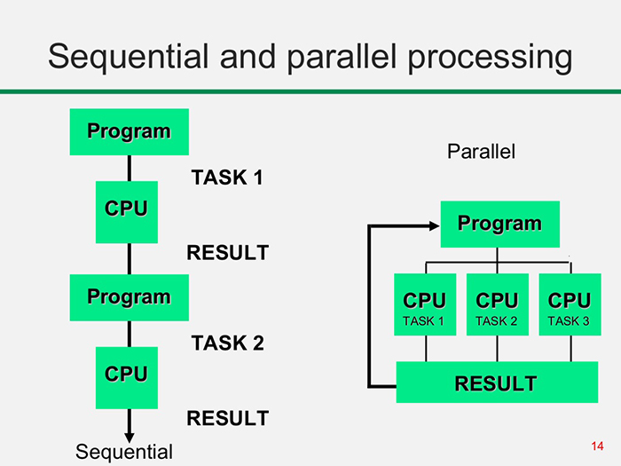
Figure 1: Illustration of sequential vs. parallel processing. Credit: https://itrelease.com/2017/11/difference-serial-parallel-processing/

As computational demands grow, parallel programming has become increasingly essential. From protein folding in drug discovery to simulations of galaxy formation and evolution, many complex problems in science rely on parallel computing. Parallel programming, hardware architecture, and systems administration intersect in the multidisciplinary field of high-performance computing (HPC). Unlike running code locally on a personal computer, HPC typically involves connecting to a cluster of networked computers, sometimes located all over the world, designed to work together on large-scale tasks.

The efficiency of a supercomputer in application to different tasks depends not only on the number of processors it carries aboard, but also on its architecture (or, in case of a cluster, on the network architecture). In this episode, we’ll briefly consider the terminology and classifications used to describe supercomputers of different types.

Computer Architectures

Historically, computer architectures are often classified into two categories: von Neumann and Harvard.
In the von Neumann design, a computer system contains the following components:

• Arithmetic/logic unit (ALU)
• Control unit (CU)
• Memory unit (MU)
• Input/output (I/O) devices

The ALU retrieves data from the MU and performs calculations, while the CU interprets instructions and directs the flow of data to and from the I/O devices, as shown in the diagram below.
In this architecture, the MU stores both data and instructions, which creates a performance bottleneck due to limited data transfer bandwidth, commonly referred to as the von Neumann bottleneck.

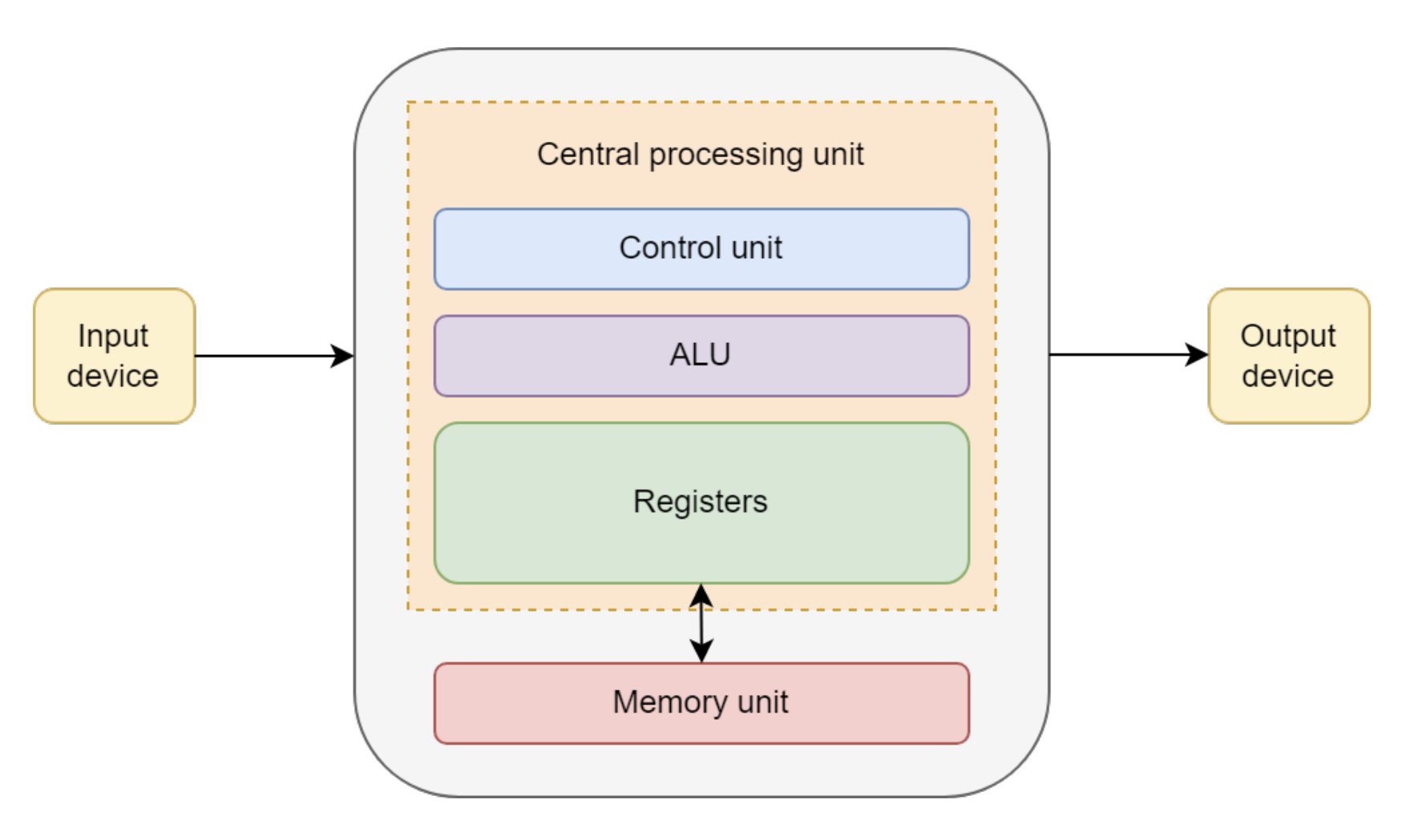
Figure 2: Diagram of von Neumann architecture, from https://onlinelibrary.wiley.com/doi/book/10.1002/9780470932025

The Harvard architecture is a variant of the von Neumann design in which instruction and data storage are physically separated.
This allows simultaneous access to both instructions and data, partially overcoming the von Neumann bottleneck.

Most modern central processing units (CPUs) use a modified Harvard architecture, in which instructions and data have separate caches but share the same main memory.
This hybrid approach combines some of the performance benefits of Harvard with the flexibility of von Neumann.

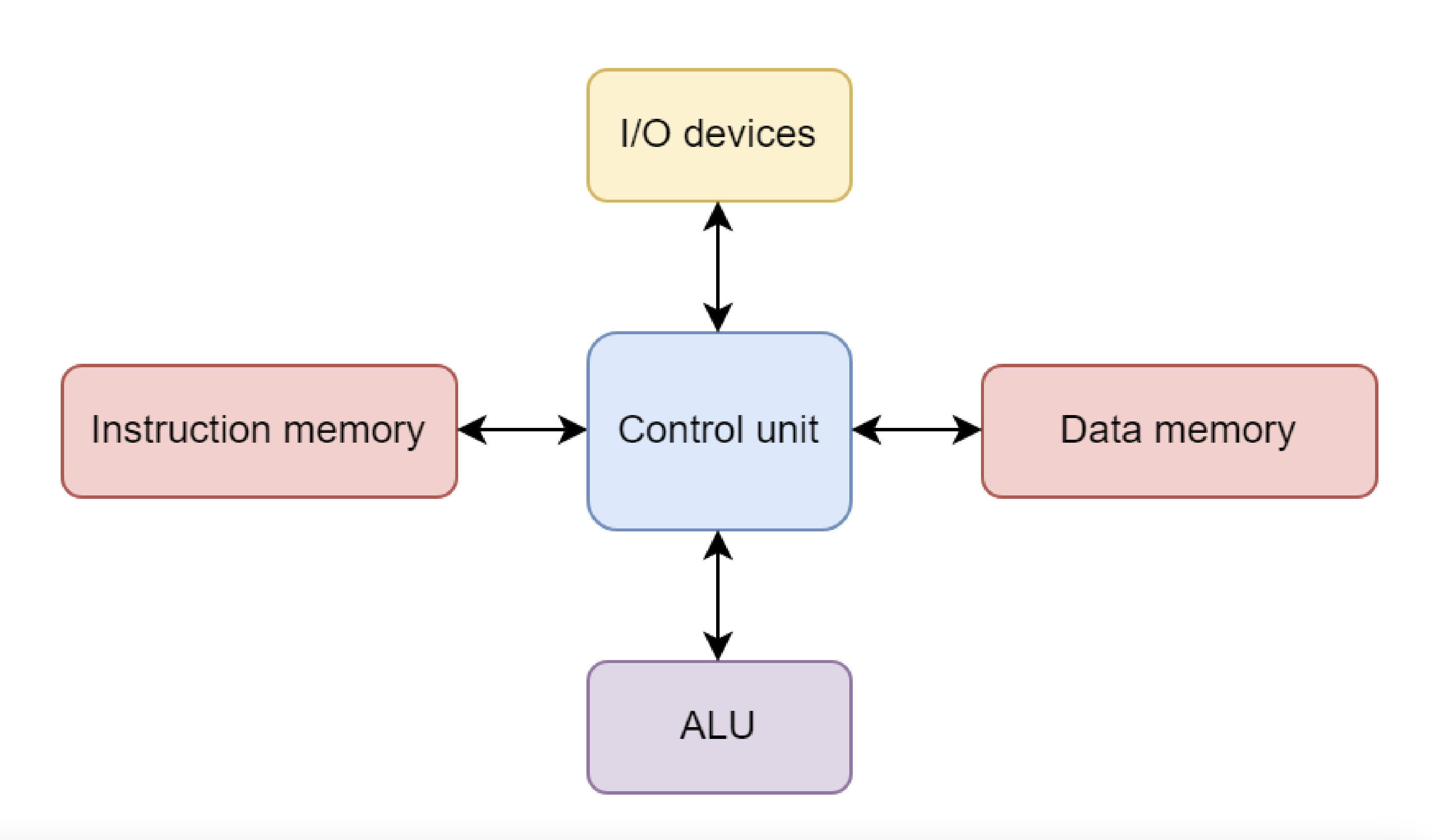
Figure 3: Diagram of Harvard architecture, from https://onlinelibrary.wiley.com/doi/book/10.1002/9780470932025

Performance

Three main components have the greatest impact on computational performance:

• CPU: CPU performance is often quantified by frequency, or “clock speed,” which determines how quickly a CPU executes instructions in terms of cycles per second. For example, a CPU with a clock speed of 3.5 GHz performs 3.5 billion cycles each second. Many CPUs have multiple cores, enabling parallel execution of multiple instructions simultaneously (Intel).

• RAM: Random access memory (RAM) is a computer’s short-term memory, storing the data needed to run applications and open files. Faster RAM allows data to move to and from the CPU more quickly, and larger RAM capacity enables the CPU to handle more complex operations simultaneously (Intel).

• Hard drive: In contrast to RAM, a computer’s hard drive is used for long-term data storage. Hard drives are characterized by both their capacity and performance. Higher-capacity drives can store more data, while higher-performance drives can read and write data faster. Hard disk drives (HDDs) generally offer more capacity for a lower cost, whereas solid state drives (SSDs) provide better performance and reliability.

Processing astronomical data, building models, and running simulations requires significant computational power. The laptop or PC you are using right now likely has between 8 GB and 32 GB of RAM, a processor with 4–10 cores, and a hard drive that can store 256 GB–1 TB of data. But what if you need to process a dataset larger than 1 TB, or load a model into RAM that exceeds 32 GB, or run a simulation that would take a month to complete on your CPU? In that case, you need a bigger computer or many computers working in parallel.

Flynn’s Taxonomy: A Framework for Parallel Computing

When discussing parallel computing, it is helpful to have a framework for classifying different types of computer architectures. The most widely used is Flynn’s Taxonomy, proposed in 1966 (Flynn, 1966). It provides a simple vocabulary for describing how computers handle tasks and will help us understand why certain programming models are better suited to certain problems.

Flynn’s taxonomy is based on four terms:

• Single
• Instruction
• Multiple
• Data

These combine to define four main architectures (HiPowered book):

• SISD (Single Instruction, Single Data): A traditional serial computer, also called a von Neumann machine. It executes one instruction at a time on a single piece of data. A laptop running a simple, non-parallel program is operating in SISD mode.
• SIMD (Single Instruction, Multiple Data): A parallel architecture in which multiple processors execute the same instruction simultaneously, but each works on a different piece of data. This approach enables massive data parallelism.
• MISD (Multiple Instruction, Single Data): Each processor executes a different instruction on the same piece of data. This architecture is very uncommon.
• MIMD (Multiple Instruction, Multiple Data): The most common type of parallel computer today. Multiple processors execute different instructions on different data at the same time. Multi-core processors, like the one sitting in your PC, and computing clusters fall into this category.

In addition to these categories, parallel computers can also be organized by memory model:

1. Multiprocessors: Shared-memory systems in which all processors access a single, unified memory space. Communication between processors occurs via this shared memory, which can simplify programming but may lead to data access errors if many processors try to use the same data simultaneously. Cores within the same processor in a personal PC use this memory system.
2. Multicomputers: Distributed-memory systems in which each processor has its own private memory. Processors communicate by passing messages over a network, which avoids memory contention but requires explicit communication management in software. This is how memory is handled in clusters.

SIMD in Practice: GPUs

A key modern example of SIMD architecture is the GPU (Graphics Processing Unit).

GPUs were originally designed for computer graphics—an inherently parallel task (e.g., calculating the color of millions of pixels at once). Researchers soon realized this massive parallelism could also be applied to general-purpose scientific computing, such as physics simulations and training AI models, leading to the term GPGPU (General-Purpose GPU). These architectures offer significant speedups for data-parallel workloads. The trade-off is that GPUs have a different memory hierarchy than CPUs, with less cache per core, so performance can be limited for algorithms that require frequent or irregular communication between threads.

A CPU consists of a small number of powerful cores optimized for complex, sequential tasks. A GPU, in contrast, contains thousands of simpler cores optimized for high-throughput, data-parallel problems. For this reason, nearly all modern supercomputers are hybrid systems that combine CPUs and GPUs, leveraging the strengths of each.

Supercomputers vs. Computing Clusters

In the early days of HPC, a “supercomputer” was typically a single, monolithic machine with custom vector processors. Today, the vast majority of systems are clusters.

• Cluster: A collection of many individual computers, so-called nodes, connected by a high-bandwidth network. Early clusters were built from single-core SISD machines, but modern nodes are almost always MIMD systems.
• Node: A single computer within the cluster. It has its own processors (CPUs), memory (RAM), and often accelerators (GPUs).
• Workload Manager (Scheduler): Software that manages the entire cluster, such as SLURM or PBS. It allocates resources, handles the job queue, and decides when and where jobs run. When you submit a job, the scheduler reserves a set of nodes for a specific time.

Network Topology for Clusters

Since a cluster is a collection of nodes, the characteristics of the connections between them, namely, the bandwidth and the network topology, is critical to performance. If a program requires frequent communication between nodes, a slow or inefficient network will cause major bottlenecks.

The most common HPC topologies are meshes, where nodes are arranged in a two- or three-dimensional grid, with each node connected to its nearest neighbors. Figure 3 shows examples of a 2D mesh, a 3D mesh, and a 2D torus (where the edges wrap around to connect boundaries, forming a torus).

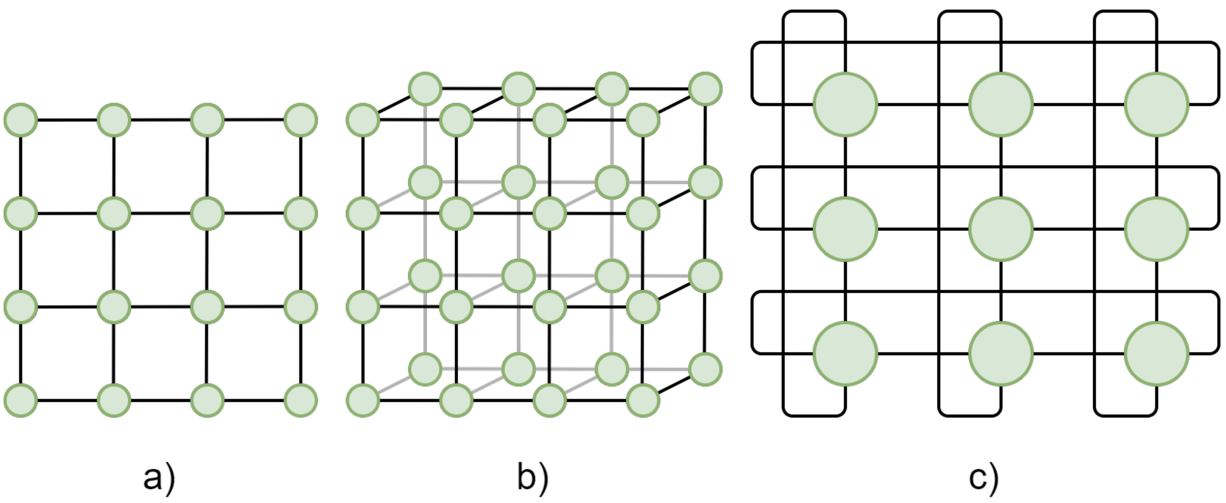
Figure 4: 2D and 3D meshes: a) 2D mesh, b) 3D mesh, c) 2D torus.

Less common HPC topologies include bus, ring, star, hypercube, tree, fully connected, crossbar, and multistage interconnection networks. These topologies are less favorable for general purpose tasks but compute clusters designed for specific use cases may adopt these designs.

HPC networks are also separated into a user-facing front end and a computational back end. The networked compute nodes like those shown in Figure 4 are part of the back end and cannot be accessed directly by the user. Users instead interact with a login node when they conect to an HPC cluster. Here, users can submit jobs to the compute nodes via a workload manager (e.g. sbatch in SLURM).

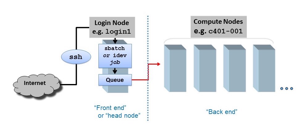
Figure 5: Separation between cluster front end and back end. Credit: https://docs.tacc.utexas.edu/basics/conduct/

Never Run Computations on the Login Node!

When you connect to an HPC cluster, you land on a login node. This shared resource is for compiling resource-light code, managing files, and submitting jobs to the workload manager, but not for heavy computation.
Running an intensive program on the login node will slow it down for everyone, and is a classic mistake for new users.
Submit your job through the workload manager so it runs on compute nodes.

File System

HPC clusters typically provide multiple storage locations, each serving different purposes:

• Home directories: Personal storage for each user, usually with limited capacity. Suitable for scripts, configuration files, and small datasets.
• Scratch: Temporary high-capacity storage for active jobs. Not backed up and typically cleared after job completion. Ideal for:
  • Jobs requiring large storage during execution
  • Datasets too large for personal storage but not needed permanently
  • Jobs needing higher-performance storage than personal directories
• Shared: Storage accessible to multiple users, often for research groups. Commonly used as a shared working directory and generally backed up regularly.

Other types of storage

Large HPC facilities may have a more complex storage organization. For example, there may exist project and archive storages, dedicated to storing large volumes of data that are not accessed often and can tolerate large lags of access time. One of the slowest, but also cheapest and most reliable storage types are magnetic tape libraries. They are commonly used for storing archival (processed with obsolete versions of pipelines) data releases of astronomical surveys, and this system is to be implemented for LSST as well. Always refer to the HPC documentation to understand how storage is implemented in this particular facility - see e.g. Iowa State University or Dartmouth HPC documentation.

Key Points

• Communication between different computer components, such as memory and arithmetic/logic unit (ALU), and between different nodes (computers) in a cluster, is often the main bottleneck of the system.

• Modern supercomputers are usually assembled from the same parts as personal computers, however, the difference is in the numbers of CPUs, GPUs and memory units, and in the way how they are connected to one another.

• Data storage organization varies from one HPC facility to another, so it is necessary to consult documentation when starting the work on a new supercomputer or cluster.

• Login nodes must not be used for computationally heavy tasks, as it will slow down the work for all users of the cluster.