Integrated Software Development Environments

Overview

Teaching: 25 min
Exercises: 15 min

Questions

• What are Integrated Development Environments (IDEs)?

• What are the advantages of using IDEs for software development?

• How does Jupyter Lab interact with virtual environments?

Objectives

• Set up Jupyter Lab and its kernels

• Use Jupyter Lab to run a script

Introduction

As we have seen in the previous episode - even a simple software project is typically split into smaller functional units and modules, which are kept in separate files and subdirectories. As your code starts to grow and becomes more complex, it will involve many different files and various external libraries. You will need an application to help you manage all the complexities of, and provide you with some useful (visual) facilities for, the software development process. Such clever and useful graphical software development applications are called Integrated Development Environments (IDEs).

Integrated Development Environments

An IDE normally consists of at least a source code editor, build automation tools and a debugger. The boundaries between modern IDEs and other aspects of the broader software development process are often blurred. Nowadays IDEs also offer version control support, tools to construct graphical user interfaces (GUI) and web browser integration for web app development, source code inspection for dependencies and many other useful functionalities. The following is a list of the most commonly seen IDE features:

• syntax highlighting - to show the language constructs, keywords and the syntax errors with visually distinct colours and font effects
• code completion - to speed up programming by offering a set of possible (syntactically correct) code options
• code search - finding package, class, function and variable declarations, their usages and referencing
• version control support - to interact with source code repositories
• debugging - for setting breakpoints in the code editor, step-by-step execution of code and inspection of variables

IDEs are extremely useful and modern software development would be very hard without them. There are a number of IDEs available for Python development; a good overview is available from the Python Project Wiki. In addition to IDEs, there are also a number of code editors that have Python support. Code editors can be as simple as a text editor with syntax highlighting and code formatting capabilities (e.g., GNU EMACS, Vi/Vim). Most good code editors can also execute code and control a debugger, and some can also interact with a version control system. Compared to an IDE, a good dedicated code editor is usually smaller and quicker, but often less feature-rich. You will have to decide which one is the best for you - in this course, we will use Jupyter Lab - a free open-source web-based IDE familiar to most Python-coding astronomers.

Is Jupyter Lab an IDE?

For a long time, Jupyter Notebook was not considered as a full-fledged IDE. The main argument against considering Jupyter Notebooks an IDE was that it lacked a lot of functionality that is essential for the full cycle of software development. The most notable instrument that wasn’t present in Jupyter Notebook was the debugger.

However, modern versions of Jupyter Lab, an evolutionary development of Jupyter Notebook, come with the built-in debugger, as well as with all the rest of the basic IDE instruments. Formally, this makes Jupyter Lab a ‘real’ IDE. At the same time, Jupyter Lab and classic IDEs (such as PyCharm or Spyder) impose distinctly different coding routines. Jupyter Lab (as Jupyter Notebook before) assumes an interactive cell-by-cell development and execution of the code, which is well-suited for data exploration and analysis and for small-scale software development. At the same time, for larger projects that do not require executing small parts of the code separately, ‘classic’ IDEs are more suitable.

Using Jupyter Lab

Let’s open our project in Jupyter Lab now and familiarise ourselves with some commonly used features.

Jupyter Lab interface

To launch Jupyter Lab, activate the venv environment created in the previous episode and type in the terminal:

 (venv) $ jupyter lab

The output will look similar to this:

 To access the server, open this file in a browser:
        file:///home/alex/.local/share/jupyter/runtime/jpserver-2946113-open.html
    Or copy and paste one of these URLs:
        http://localhost:8888/lab?token=e2aff7125e9917868a16b8b627f73995eb83effbcafeee05
        http://127.0.0.1:8888/lab?token=e2aff7125e9917868a16b8b627f73995eb83effbcafeee05

Now you can click on one of the URLs below and Jupyter Lab will open in your browser.

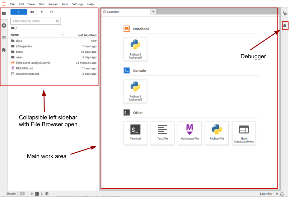
Jupyter Lab starting interface

The Jupyter Lab interface includes the following areas:

1. Menu bar, from which you can access most common Jupyter Lab functions;
2. A collapsible left sidebar, in which four tabs are present:
   • File Manager. From here you can manage the files and directories in your repository folder.
   • Running terminal and kernels. Here you can find the list of running Jupyter Notebook kernels and console sessions.
   • Table of contents. Here Jupyter Lab will automatically generate a table of contents of your notebooks (using headers and other markdown cells) and Python files (using function and class definitions).
   • Extension Manager. In this section, it is possible to install extensions that expand Jupyter Lab functionality, for example, allowing integration with Git, adding CSS formatting, and so on.
3. The main work area. When you just opened Jupyter Lab, you can see several options for starting your work, such as creating a new Notebook, opening a new Python console session, or creating a new text or Python file. The list of these options will vary depending on which kernels and programming languages you have installed. When you open a Notebook or a file, it will appear in a separate tab in this area.
4. In the right collapsible sidebar you can access the notebooks’ Properties Manager and Debugger, which can be used for inspecting the variables and managing Breakpoints.

Opening a Software Project

In the left sidebar, open the File Browser and look through the files present here. You can inspect the requirements.txt file, where we saved the list of packages installed in our virtual environment, and README.md, containing some basic information about the project. Later we will add more information to this file. For now, double click on the light-curve-analysis.ipynb.

In the opened tab we can see a number of cells. Some of them contain Python code, while others display formatted text (‘Markdown’). You can change the type of the cell in the drop-down menu in the instrumental panel on the top of the tab. You can execute cells one by one by pressing Shift+Enter, or run them all by choosing Run > Run All in the main menu or by pressing a corresponding button in the tab instrumental panel. Code cells produce outputs, which may contain text, tables and static or interactive plots.

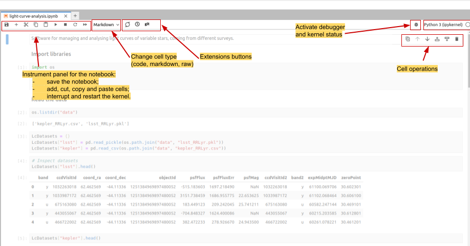
Interface elements of a notebook tab

By default the notebooks are opened in tabs that take the full screen, however, you can align them vertially or horizontally by dragging them in the preferred place. You can also place an output of any cell into a separate tab. For this, make a right-click on the output content and choose Create New View for Cell Output. You can open multiple tabs for the cell outputs and reorder them in the same way as the notebook tabs.

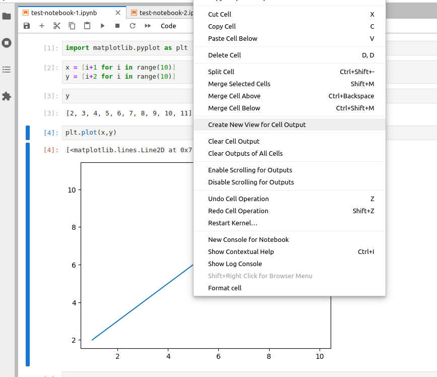
Creating cell output view

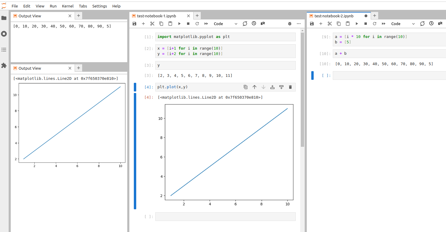
You can order the notebook tabs and cell output views any way you like

The code in the notebook is displayed using different colours, following the rules set up for the syntax highlighting. Syntax highlighting is a feature that displays source code terms in different colours and fonts according to the syntax category the highlighted term belongs to. It also makes syntax errors visually distinct. Highlighting does not affect the meaning of the code itself - it’s intended only for humans to make reading code and finding errors easier. The code highlighting color scheme depends on the programming language (or, to be more precise, on the kernel which is currently connected to your Notebook), and in the Text Editor, you can pick the language yourself in View > Text Editor Syntax Highlighting menu. By default it is inferred from the file extension, e.g. Python for .py files.

Code Completion & Documentation References

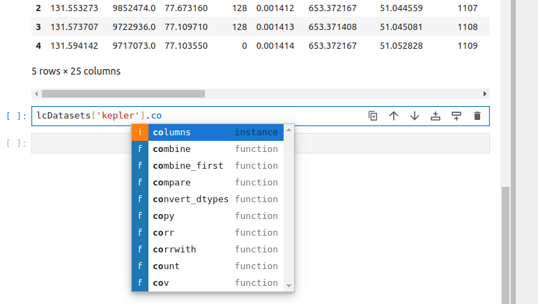
Context-aware code completion suggestions (`Tab`)

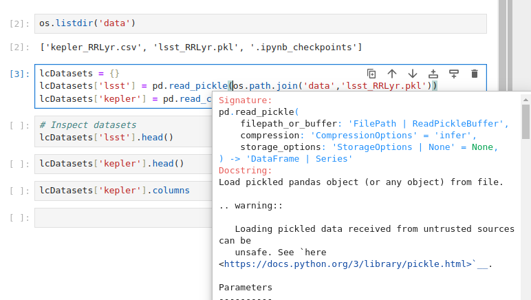
Contextual help in a pop-up window (`Shift+Tab`)

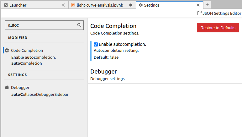
Setting up auto-completion

When you are typing code, you can use completion suggestions and contextual help tools, included in Jupyter Lab. You can use three hotkey combinations for using these tools:

1. When you start typing a command, you can press Tab, and Jupyter Lab will offer you options of code that can follow.
2. You also can type Shift+Tab to open contextual help in a pop-up window.
3. Another option is to use Ctrl+I for opening contextual help in the right sidebar.
4. Finally, you can enable code auto-completion. For this, go to ‘Settings > Settings Editor’ and start typing ‘auto-completion’ in the Search box. Then select the ‘Enable autocompletion’ checkbox.

Using context-aware code completion features speeds up the process of coding, and reduces typos and other common mistakes. Using contextual help also improves the quality of the code, as well as simplifies the process for the programmer.

How does contextual help work?

Contextual help relies on the docstrings, written in the library’s source files by the developers. If you look at code definitions of well-maintained libraries, such as Pandas or Numpy, you will see that the docstrings are very detailed: they contain input parameters, outputs, algorithm descriptions, and even examples of usage. Later we will talk about how to write good docstrings, but here you can see why they are so essential.

Try completion, auto-completion, and contextual help functions

Execute already existing cells of the notebook. There are several ways to do this:

1. You can go through the cells, clicking Shift+Enter on each of them.
2. You can use Run > Run all cells menu.
3. You can use Restart the kernel and run all cells button on the tool panel on the top of your notebook tab. Be aware that when you restart the kernel, you lose all the data from already executed code, e.g. all the variables will be deleted.

After that, inspect contextual help of several functions, e.g. pd.read_pickle, np.array, and os.path.join. Pay attention to which information is included in the contextual help and in which format. Next, get the list of the columns in one of the opened datasets, using completion at every step.

Solution

To get the list of the columns you can use the following code: LcDatasets['kepler'].columns. By pressing Tab once you started typing ‘LcDatasets’, ‘kepler’ and ‘columns’, you will get suggestions for the available options of the following code.

After that, enable auto-completion and get the list of the columns of the second dataset. Depending on what is more convenient for you, you can leave auto-completion function turned on, or turn it off.

Code Search

Jupyter Lab offers you the possibility to search and replace text within the file, using case matching and regular expressions. You can perform the search within the whole document or only in a single cell, with or without cell outputs (the results of execution of the code within the cell). To access the search tool, use Ctrl+F key combination, or Edit > Find in the main menu.

Searching across multiple notebooks

Jupyter Lab built-in search does not allow searching strings across multiple files. However, such functionality is available with jupyterlab-search-replace extension.

Jupyter Lab magic

Jupyter magic commands or simply magics are special commands, provided by the default Jupyter kernel (‘backend’ that executes the code) called IPython. Magics allow us to conveniently perform many useful operations since they can interact with operational system and Jupyter kernels. There are two types of magics: the ones that operate on a single line of the following code (the code has to be written on the same line after a single space, without parenthesis or quotation marks), and the ones that act upon the content of a whole single cell. The line magics are preceded by a single percentage symbol (%), while cell magics use two percentage symbols (%%). Here is a short list of the most useful magics:

• %magic: prints information about magics system
• %lsmagic: lists all magic commands in a convenient form
• %quickref: another helper function that shows references for the magic commands
• %time, %timeit and %%timeit: measure the execution time of the code.
• %cd, %ls, %pwd and other console commands: executes terminal commands
• %run: executes another ‘.ipynb’ or ‘.py’ file from within the current notebook
• %who: lists the defined variables. It is possible to list only variables of a certain type, e.g. %who string

%time, %timeit and %%timeit

The difference between %time and %timeit is that first command executes your code only once, while the second runs it several times and measures the average execution time, attempting to get a more precise value. However, the second command isn’t always better! For example, if you measure the execution time of a list sorting, after the first execution the list will already be sorted, and executing the same code over already sorted list will take much less time, meaning that the average execution time will be skewed towards lesser numbers. %%timeit, as follows from two ‘%’ signs, measures the execution time for all code in a cell together.

Try out different magics

Try several different magic commands, such as %lsmagic, %pwd and %who. Use %who command to get the list of dict variables (pay attention, that if you use %who command without specifying the type of the variable, it will also include the packages that you imported in the notebook).

Apart from the built-in magics, there are many more that you can install additionally. It is also possible to develop your own magic commands.

Installing packages from Jupyter notebook interface or Jupyter console session

Since magics allow us to execute terminal commands, there is a way to install Python packages right from the Jupyter interface. We can run %pip3 install astropy right in a Jupyter cell. This is a standard way of installing packages in cloud Jupyter Notebook services, such as Google Colab or the Notebook aspect of Rubin Science Platform. Pay attention, though, that another common way of doing this, using ! instead of % before the installation command, is in general not safe and can lead to the dependencies issues due to the particularities of how OS and Jupyter kernels interact. You can still see it often, since magic command for pip appeared only in the later versions of IPython.

Key Points

• An IDE is an application that provides a comprehensive set of facilities for software development, including syntax highlighting, code search and completion, version control, testing and debugging.

• Jupyter Lab launches within the pre-existing virtual environment

• We can run terminal commands within Jupyter Lab