Setting the Scene
Overview
Teaching: 15 min
Exercises: 0 minQuestions
What are we teaching in this course?
What motivated the selection of topics covered in the course?
Objectives
Setting the scene and expectations
Making sure everyone has all the necessary software installed
Introduction
So, you have gained basic software development skills either by self-learning or attending, e.g., a novice Software Carpentry course. You have been applying those skills for a while by writing code to help with your work and you feel comfortable developing code and troubleshooting problems. However, your software has now reached a point where there’s too much code to be kept in one script. Perhaps it’s involving more researchers (developers) and users, and more collaborative development effort is needed to add new functionality while ensuring previous development efforts remain functional and maintainable.
This course provides the next step in software development - it teaches some intermediate software engineering skills and best practices to help you restructure existing code and design more robust, reusable and maintainable code, automate the process of testing and verifying software correctness and support collaborations with others in a way that mimics a typical software development process within a team.
The course uses a number of different software development tools and techniques interchangeably as you would in a real life. We had to make some choices about topics and tools to teach here, based on established best practices, ease of tool installation for the audience, length of the course and other considerations. Tools used here are not mandated though: alternatives exist and we point some of them out along the way. Over time, you will develop a preference for certain tools and programming languages based on your personal taste or based on what is commonly used by your group, collaborators or community. However, the topics covered should give you a solid foundation for working on software development in a team and producing high quality software that is easier to develop and sustain in the future by yourself and others. Skills and tools taught here, while Python-specific, are transferable to other similar tools and programming languages.
The course is organised into the following sections:
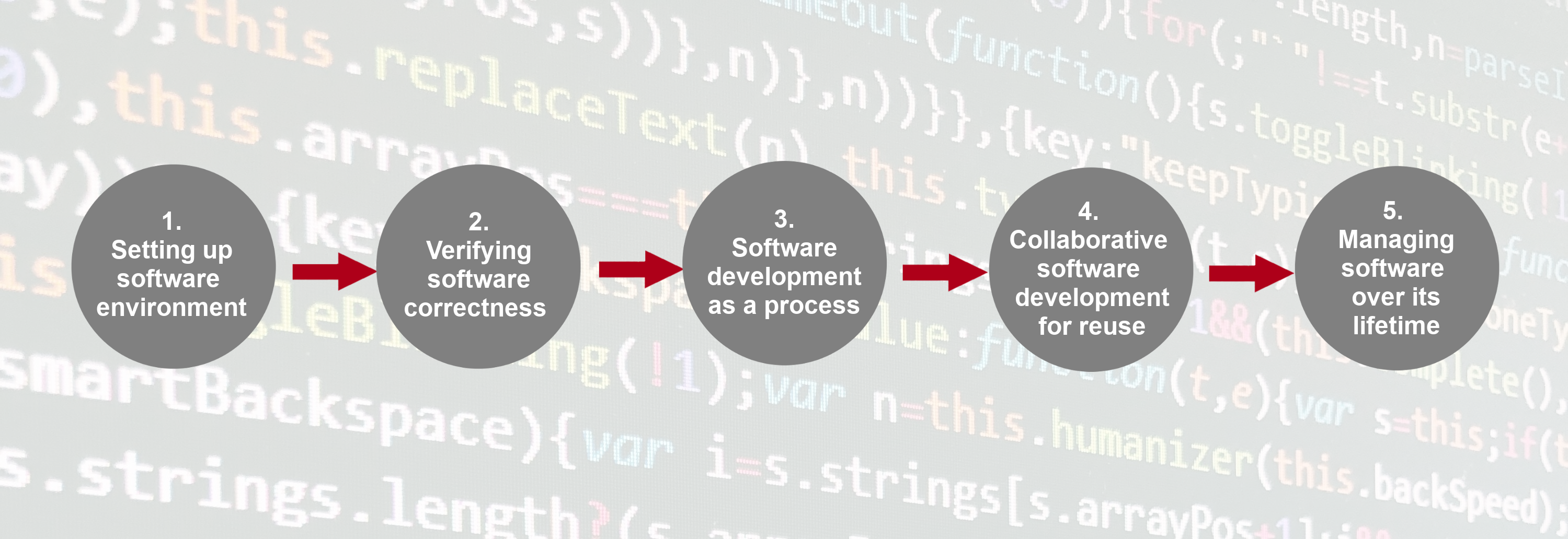
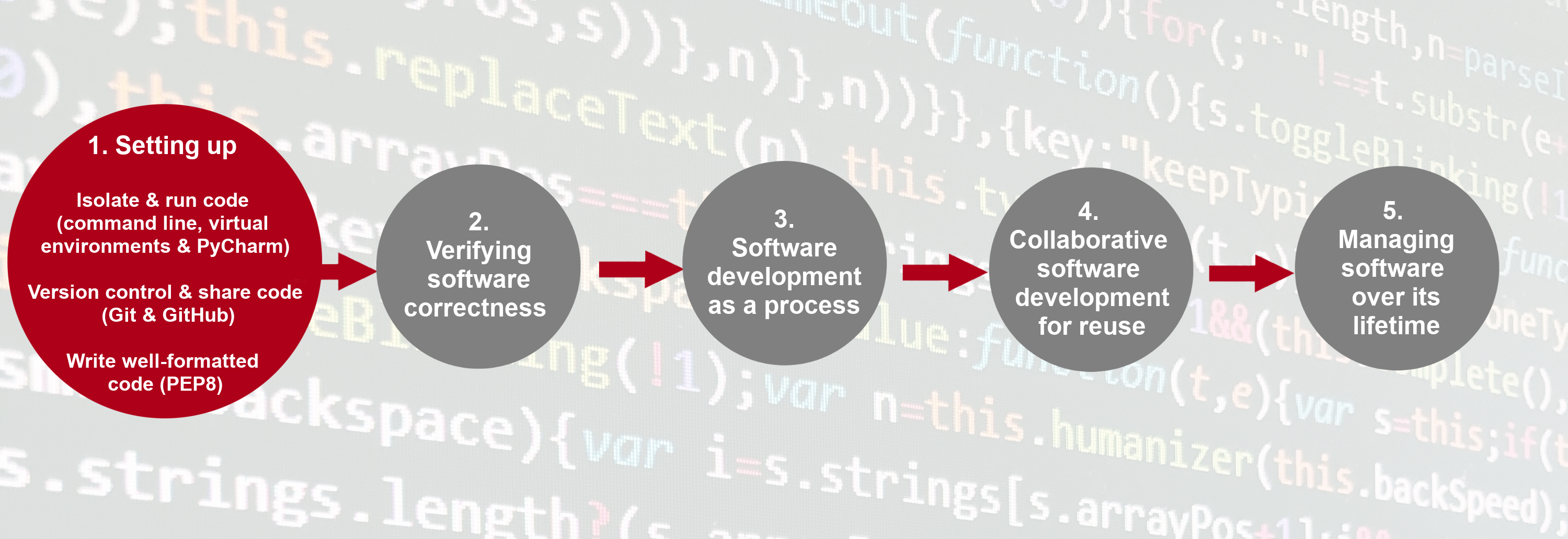
Section 1: Setting up Software Environment
In the first section we are going to set up our working environment and familiarise ourselves with various tools and techniques for software development in a typical collaborative code development cycle:
- Virtual environments for isolating a project from other projects developed on the same machine
- Command line for running code and interacting with the command line tool Git for
- Integrated Development Environment for code development, testing and debugging, Version control and using code branches to develop new features in parallel,
- GitHub (central and remote source code management platform supporting version control with Git) for code backup, sharing and collaborative development, and
- Python code style guidelines to make sure our code is documented, readable and consistently formatted.
Section 2: Verifying Software Correctness at Scale
Once we know our way around different code development tools, techniques and conventions, in this section we learn:
- how to set up a test framework and write tests to verify the behaviour of our code is correct, and
- how to automate and scale testing with Continuous Integration (CI) using GitHub Actions (a CI service available on GitHub).
Section 3: Software Development as a Process
In this section, we step away from writing code for a bit to look at software from a higher level as a process of development and its components:
- different types of software requirements and designing and architecting software to meet them, how these fit within the larger software development process and what we should consider when testing against particular types of requirements.
- different programming and software design paradigms, each representing a slightly different way of thinking about, structuring and implementing the code.
Section 4: Collaborative Software Development for Reuse
Advancing from developing code as an individual, in this section you will start working with your fellow learners on a group project (as you would do when collaborating on a software project in a team), and learn:
- how code review can help improve team software contributions, identify wider codebase issues, and increase codebase knowledge across a team.
- what we can do to prepare our software for further development and reuse, by adopting best practices in documenting, licencing, tracking issues, supporting your software, and packaging software for release to others.
Section 5: Managing and Improving Software Over Its Lifetime
Finally, we move beyond just software development to managing a collaborative software project and will look into:
- internal planning and prioritising tasks for future development using agile techniques and effort estimation, management of internal and external communication, and software improvement through feedback.
- how to adopt a critical mindset not just towards our own software project but also to assess other people’s software to ensure it is suitable for us to reuse, identify areas for improvement, and how to use GitHub to register good quality issues with a particular code repository.
Before We Start
A few notes before we start.
Prerequisite Knowledge
This is an intermediate-level software development course intended for people who have already been developing code in Python (or other languages) and applying it to their own problems after gaining basic software development skills. So, it is expected for you to have some prerequisite knowledge on the topics covered, as outlined at the beginning of the lesson. Check out this quiz to help you test your prior knowledge and determine if this course is for you.
Setup, Common Issues & Fixes
Have you setup and installed all the tools and accounts required for this course? Check the list of common issues, fixes & tips if you experience any problems running any of the tools you installed - your issue may be solved there.
Compulsory and Optional Exercises
Exercises are a crucial part of this course and the narrative. They are used to reinforce the points taught and give you an opportunity to practice things on your own. Please do not be tempted to skip exercises as that will get your local software project out of sync with the course and break the narrative. Exercises that are clearly marked as “optional” can be skipped without breaking things but we advise you to go through them too, if time allows. All exercises contain solutions but, wherever possible, try and work out a solution on your own.
Outdated Screenshots
Throughout this lesson we will make use and show content from Graphical User Interface (GUI) tools (Jupyter Lab and GitHub). These are evolving tools and platforms, always adding new features and new visual elements. Screenshots in the lesson may then become out-of-sync, refer to or show content that no longer exists or is different to what you see on your machine. If during the lesson you find screenshots that no longer match what you see or have a big discrepancy with what you see, please open an issue describing what you see and how it differs from the lesson content. Feel free to add as many screenshots as necessary to clarify the issue.
Let Us Know About the Issues
The original materials were adapted specifically for this workshop. They weren’t used before, and it is possible that they contain typos, code errors, or underexplained or unclear moments. Please, let us know about these issues. It will help us to improve the materials and make the next workshop better.
Key Points
This lesson focuses on core, intermediate skills covering the whole software development life-cycle that will be of most use to anyone working collaboratively on code.
For code development in teams - you need more than just the right tools and languages. You need a strategy (best practices) for how you’ll use these tools as a team.
The lesson follows on from the novice Software Carpentry lesson, but this is not a prerequisite for attending as long as you have some basic Python, command line and Git skills and you have been using them for a while to write code to help with your work.
Section 1: Setting Up Environment For Collaborative Code Development
Overview
Teaching: 10 min
Exercises: 0 minQuestions
What tools are needed to collaborate on code development effectively?
Objectives
Provide an overview of all the different tools that will be used in this course.
The first section of the course is dedicated to setting up your environment for collaborative software development and introducing the project that we will be working on throughout the course. In order to build working (research) software efficiently and to do it in collaboration with others rather than in isolation, you will have to get comfortable with using a number of different tools interchangeably as they’ll make your life a lot easier. There are many options when it comes to deciding which software development tools to use for your daily tasks - we will use a few of them in this course that we believe make a difference. There are sometimes multiple tools for the job - we select one to use but mention alternatives too. As you get more comfortable with different tools and their alternatives, you will select the one that is right for you based on your personal preferences or based on what your collaborators are using.
Here is an overview of the tools we will be using.
Setup, Common Issues & Fixes
Have you setup and installed all the tools and accounts required for this course? Check the list of common issues, fixes & tips if you experience any problems running any of the tools you installed - your issue may be solved there.
Command Line & Python Virtual Development Environment
We will use the command line
(also known as the command line shell/prompt/console)
to run our Python code
and interact with the version control tool Git and software sharing platform GitHub.
We will also use command line tools
venv
and pip
to set up a Python virtual development environment
and isolate our software project from other Python projects we may work on.
Note: some Windows users experience the issue where Python hangs from Git Bash
(i.e. typing python causes it to just hang with no error message or output) -
see the solution to this issue.
Integrated Development Environment (IDE)
An IDE integrates a number of tools that we need to develop a software project that goes beyond a single script - including a smart code editor, a code compiler/interpreter, a debugger, etc. It will help you write well-formatted and readable code that conforms to code style guides (such as PEP8 for Python) more efficiently by giving relevant and intelligent suggestions for code completion and refactoring. IDEs often integrate command line console and version control tools - we teach them separately in this course as this knowledge can be ported to other programming languages and command line tools you may use in the future (but is applicable to the integrated versions too).
There are several popular IDEs for Python, such as IDLE, PyCharm, Spyder, VS Studio, and so on. In this course, we will use Jupyter Lab - a free, open-source IDE, widely used in the astronomic community.
Is JupyterLab actually an IDE?
JupyterLab is the next evolutionary step for the Jupyter Notebooks, a web-based interactive environment for exploratory coding. While Jupyter Notebooks lack some of the features of classical IDEs (most notably, a debugger), the latest versions of JupyterLab include all the necessary functionality. Terminology aside, JupyterLab is a very popular tool for data analysis and in the research community. More so, JupyterLab still bears a strong resemblance to Jupyter Notebooks, Google Colab and LSST Rubin Science Platform (RSP) Notebook aspect. Many astronomical platforms that provide access to computational resources and observational datasets also have Jupyter Notebooks installed. For this reason, in this course, we aim to show which tools and practices can help you write high-quality, reusable, and reliable software using JupyterLab. The original version of this course was developed for PyCharm IDE, which is usually considered to be more suited for software development that is not related to data exploration and analysis. That course is included in the Carpentries Incubator program, and you can access it here.
Git & GitHub
Git is a free and open source distributed version control system designed to save every change made to a (software) project, allowing others to collaborate and contribute. In this course, we use Git to version control our code in conjunction with GitHub for code backup and sharing. GitHub is one of the leading integrated products and social platforms for modern software development, monitoring and management - it will help us with version control, issue management, code review, code testing/Continuous Integration, and collaborative development. An important concept in collaborative development is version control workflows (i.e. how to effectively use version control on a project with others).
Python Coding Style
Most programming languages will have associated standards and conventions for how the source code should be formatted and styled. Although this sounds pedantic, it is important for maintaining the consistency and readability of code across a project. Therefore, one should be aware of these guidelines and adhere to whatever the project you are working on has specified. In Python, we will be looking at a convention called PEP8.
Let’s get started with setting up our software development environment!
Key Points
In order to develop (write, test, debug, backup) code efficiently, you need to use a number of different tools.
When there is a choice of tools for a task you will have to decide which tool is right for you, which may be a matter of personal preference or what the team or community you belong to is using.
Introduction to Our Software Project
Overview
Teaching: 20 min
Exercises: 10 minQuestions
What is the design architecture of our example software project?
Why is splitting code into smaller functional units (modules) good when designing software?
Objectives
Use Git to obtain a working copy of our software project from GitHub.
Inspect the structure and architecture of our software project.
Understand Model-View-Controller (MVC) architecture in software design and its use in our project.
Light Curve Analysis Project
For this workshop, let’s assume that you have joined a software development team that has been working on the light curve analysis project developed in Python and stored on GitHub. The purpose of this software is to analyze the variability of astronomical sources, using observations that come from different instruments.

What Does Light Curve Dataset Contain?
For developing and testing our software project, we will use two RR Lyrae candidates variability datasets.
The first dataset,
kepler_RRLyr.csv, contains observations coming from the Kepler space telescope. In this dataset, all observations are related to the same source, i.e. the whole table represents a single light curve. The second dataset,lsst_RRLyr.pkl, contains synthetic observations of 25 presumably variable sources from the LSST Data Preview 0. Considering that the datasets come from different instruments, they also have different formats and column names - a common situation in real life. It is always a good idea to develop your software in such a way that it remains usable even if the format of the input data has changed. We will use the differences of the datasets to illustrate some of the topics during this workshop.
The project is not finished and contains some errors. You will be working on your own and in collaboration with others to fix and build on top of the existing code during the course.
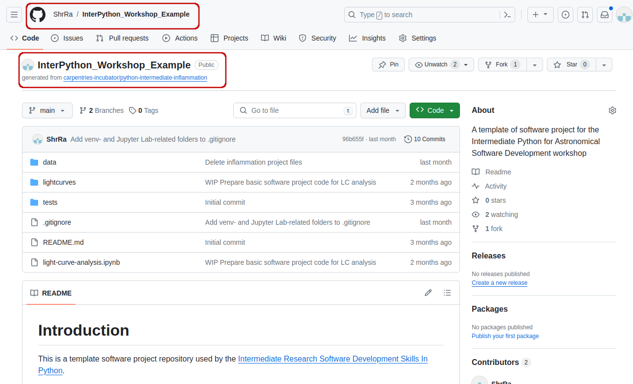
Downloading Our Software Project
To start working on the project, you will first create a copy of the software project template repository from GitHub within your own GitHub account and then obtain a local copy of that project (from your GitHub) on your machine.
- Make sure you have a GitHub account and that you have set up your SSH key pair for authentication with GitHub, as explained in Setup.
- Log into your GitHub account.
-
Go to the software project repository in GitHub.

-
Click the
Forkbutton towards the top right of the repository’s GitHub page to create a fork of the repository under your GitHub account. Remember, you will need to be signed into GitHub for theForkbutton to work.Note: each participant is creating their own fork of the project to work on.
-
Make sure to select your personal account and set the name of the project to
InterPython_Workshop_Example(you can call it anything you like, but it may be easier for future group exercises if everyone uses the same name). Also set the new repository’s visibility to ‘Public’ - so it can be seen by others and by third-party Continuous Integration (CI) services (to be covered later on in the course) and select theCopy the main branch onlycheckbox.
- Click the
Create forkbutton and wait for GitHub to import the copy of the repository under your account. -
Locate the forked repository under your own GitHub account. GitHub should redirect you there automatically after creating the fork. If this does not happen, click your user icon in the top right corner and select Your Repositories from the drop-down menu, then locate your newly created fork.
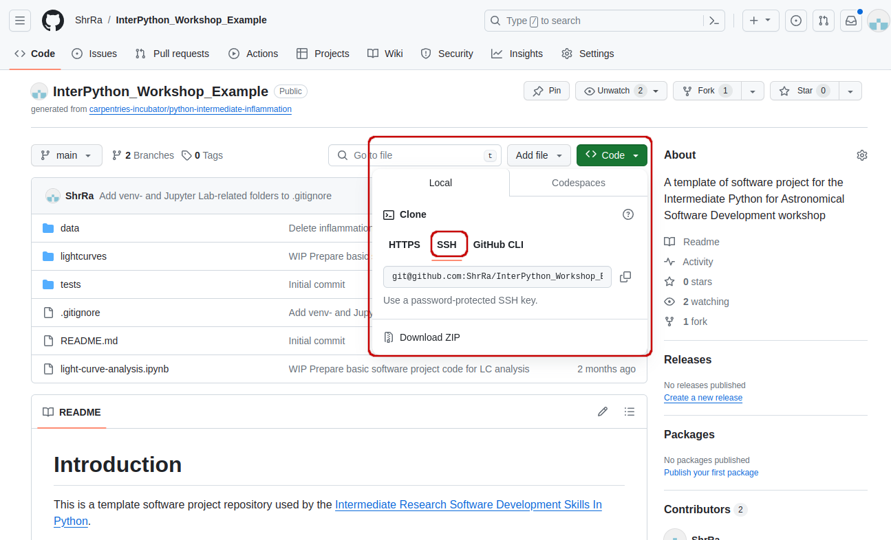
Exercise: Obtain the Software Project Locally
Using the command line, clone the copied repository from your GitHub account into the home directory on your computer using SSH. Which command(s) would you use to get a detailed list of contents of the directory you have just cloned?
Solution
- Find the SSH URL of the software project repository to clone from your GitHub account. Make sure you do not clone the original template repository but rather your own copy, as you should be able to push commits to it later on. Also make sure you select the SSH tab and not the HTTPS one. These two protocols implement different security measures, and since 2021 GitHub offers full support only for the SSH cloning; namely, you won’t be able to send your changes to the repository if you use HTTPS method.
- Make sure you are located in your home directory in the command line with:
$ cd ~- From your home directory in the command line, do:
$ git clone git@github.com:<YOUR_GITHUB_USERNAME>/InterPython_Workshop_Example.gitMake sure you are cloning your copy of the software project and not the template repository.
- Navigate into the cloned repository folder in your command line with:
$ cd InterPython_Workshop_ExampleNote: If you have accidentally copied the HTTPS URL of your repository instead of the SSH one, you can easily fix that from your project folder in the command line with:
$ git remote set-url origin git@github.com:<YOUR_GITHUB_USERNAME>/InterPython_Workshop_Example.git
Our Software Project Structure
Let’s inspect the content of the software project from the command line.
From the root directory of the project,
you can use the command ls -l to get a more detailed list of the contents.
You should see something similar to the following.
$ cd ~/InterPython_Workshop_Example
$ ls -l
total 284
drwxrwxr-x 2 alex alex     52 Jan 10 20:29 data
-rw-rw-r-- 1 alex alex 285218 Jan 10 20:29 light-curve-analysis.ipynb
drwxrwxr-x 2 alex alex     58 Jan 10 20:29 lcanalyzer
-rw-rw-r-- 1 alex alex   1171 Jan 10 20:29 README.md
drwxrwxr-x 2 alex alex     51 Jan 10 20:29 tests
...
As can be seen from the above, our software project contains the README file
(that typically describes the project, its usage, installation, authors and how to contribute),
Jupyter Notebook light-curve-analysis.ipynb, and three directories - lcanalyzer, data and tests.
The Jupyter Notebook light-curve-analysis.ipynb is where exploratory analysis is done,
and on closer inspection, we can see that the lcanalyzer directory contains two Python
scripts - views.py and models.py. We will have a more detailed look into these shortly.
$ cd ~/InterPython_Workshop_Example/lcanalyzer
$ ls -l
total 12
-rw-rw-r-- 1 alex alex 903 Jan 10 20:29 models.py
-rw-rw-r-- 1 alex alex 718 Jan 10 20:29 views.py
...
Directory data contains three files with the lightcurves coming from two instruments, Kepler and LSST:
$ cd ~/InterPython_Workshop_Example/data
$ ls -l
total 24008
-rw-rw-r-- 1 alex alex 23686283 Jan 10 20:29 kepler_RRLyr.csv
-rw-rw-r-- 1 alex alex   895553 Jan 10 20:29 lsst_RRLyr.pkl
-rw-rw-r-- 1 alex alex   895553 Jan 10 20:29 lsst_RRLyr_protocol_4.pkl
...
The lsst_RRLyr_protocol_4.pkl file contains the same data as lsst_RRLyr.pkl, but it’s saved
using an older data protocol, compatible with older versions of the packages we’ll be using.
Exercise: Have a Peek at the Data
Which command(s) would you use to list the contents or a first few lines of
data/kepler_RRLyr.csvfile?Solution
- To list the entire content of a file from the project root do:
cat data/kepler_RRLyr.csv.- To list the first 5 lines of a file from the project root do:
head -n 5 data/kepler_RRLyr.csv.time,flux,flux_err,quality,timecorr,centroid_col,centroid_row,cadenceno,sap_flux,sap_flux_err,sap_bkg,sap_bkg_err,pdcsap_flux,pdcsap_flux_err,sap_quality,psf_centr1,psf_centr1_err,psf_centr2,psf_centr2_err,mom_centr1,mom_centr1_err,mom_centr2,mom_centr2_err,pos_corr1,pos_corr2 ...Pay attention that while the
.csvformat is human-readable, if you try to runhead -n 5 data/lsst_RRLyr.pkl, the output will be non-human-readable.
Directory tests contains several tests that have been implemented already.
We will be adding more tests during the course as our code grows.
$ ls -l tests
total 8
-rw-rw-r-- 1 alex alex 941 Jan 10 20:29 test_models.py
...
An important thing to note here is that the structure of the project is not arbitrary. One of the big differences between novice and intermediate software development is planning the structure of your code. This structure includes software components and behavioural interactions between them (including how these components are laid out in a directory and file structure). A novice will often make up the structure of their code as they go along. However, for more advanced software development, we need to plan this structure - called a software architecture - beforehand.
Let’s have a more detailed look into what a software architecture is and which architecture is used by our software project before we start adding more code to it.
Software Architecture
A software architecture is the fundamental structure of a software system that is decided at the beginning of project development based on its requirements and cannot be changed that easily once implemented. It refers to a “bigger picture” of a software system that describes high-level components (modules) of the system and how they interact.
In software design and development,
large systems or programs are often decomposed into a set of smaller modules
each with a subset of functionality.
Typical examples of modules in programming are software libraries;
some software libraries, such as numpy and matplotlib in Python,
are bigger modules that contain several smaller sub-modules.
Another example of modules are classes in object-oriented programming languages.
Programming Modules and Interfaces
Although modules are self-contained and independent elements to a large extent (they can depend on other modules), there are well-defined ways of how they interact with one another. These rules of interaction are called programming interfaces - they define how other modules (clients) can use a particular module. Typically, an interface to a module includes rules on how a module can take input from and how it gives output back to its clients. A client can be a human, in which case we also call these user interfaces. Even smaller functional units such as functions/methods have clearly defined interfaces - a function/method’s definition (also known as a signature) states what parameters it can take as input and what it returns as an output.
There are various software architectures around defining different ways of dividing the code into smaller modules with well defined roles, for example:
- Model–View–Controller (MVC) architecture, which we will look into in detail and use for our software project,
- Service-oriented architecture (SOA), which separates code into distinct services, accessible over a network by consumers (users or other services) that communicate with each other by passing data in a well-defined, shared format (protocol),
- Client-server architecture, where clients request content or service from a server, initiating communication sessions with servers, which await incoming requests (e.g. email, network printing, the Internet),
- Multilayer architecture, is a type of architecture in which presentation, application processing and data management functions are split into distinct layers and may even be physically separated to run on separate machines - some more detail on this later in the course.
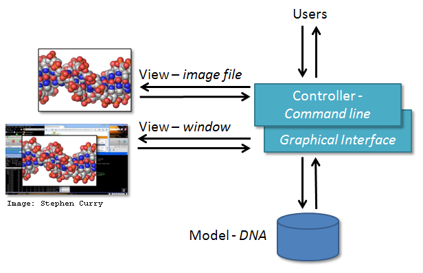
Model-View-Controller (MVC) Architecture
MVC architecture divides the related program logic into three interconnected modules:
- Model (data)
- View (client interface), and
- Controller (processes that handle input/output and manipulate the data).
Model represents the data used by a program and also contains operations/rules for manipulating and changing the data in the model. This may be a database, a file, a single data object or a series of objects - for example a table representing light curve observations.
View is the means of displaying data to users/clients within an application (i.e. provides visualisation of the state of the model). For example, displaying a window with input fields and buttons (Graphical User Interface, GUI) or textual options within a command line (Command Line Interface, CLI) are examples of Views. They include anything that the user can see from the application. While building GUIs is not the topic of this course, we will cover building CLIs in Python in later episodes.
Controller manipulates both the Model and the View. It accepts input from the View and performs the corresponding action on the Model (changing the state of the model) and then updates the View accordingly. For example, on user request, Controller updates a picture on a user’s GitHub profile and then modifies the View by displaying the updated profile back to the user.
MVC Examples
MVC architecture can be applied in scientific applications in the following manner. Model comprises those parts of the application that deal with some type of scientific processing or manipulation of the data, e.g. numerical algorithm, simulation, statistical analysis. View is a visualisation, or format, of the output, e.g. graphical plot, diagram, chart, data table, file. Controller is the part that ties the scientific processing and output parts together, mediating input and passing it to the model or view, e.g. command line options, mouse clicks, input files. For example, the diagram below depicts the use of MVC architecture for the DNA Guide Graphical User Interface application.
Exercise: MVC Application Examples From your Work
Think of some other examples from your work or life where MVC architecture may be suitable or have a discussion with your fellow learners.
Solution
MVC architecture is a popular choice when designing web and mobile applications. Users interact with a web/mobile application by sending various requests to it. Forms to collect users inputs/requests together with the info returned and displayed to the user as a result represent the View. Requests are processed by the Controller, which interacts with the Model to retrieve or update the underlying data. For example, a user may request to view its profile. The Controller retrieves the account information for the user from the Model and passes it to the View for rendering. The user may further interact with the application by asking it to update its personal information. Controller verifies the correctness of the information (e.g. the password satisfies certain criteria, postal address and phone number are in the correct format, etc.) and passes it to the Model for permanent storage. The View is then updated accordingly and the user sees its updated profile details.
Note that not everything fits into the MVC architecture but it is still good to think about how things could be split into smaller units. For a few more examples, have a look at this short article on MVC from CodeAcademy.
Separation of Concerns
Separation of concerns is important when designing software architectures in order to reduce the code’s complexity. Note, however, there are limits to everything - and MVC architecture is no exception. Controller often transcends into Model and View and a clear separation is sometimes difficult to maintain. For example, the Command Line Interface provides both the View (what user sees and how they interact with the command line) and the Controller (invoking of a command) aspects of a CLI application. In Web applications, Controller often manipulates the data (received from the Model) before displaying it to the user or passing it from the user to the Model.
Our Project’s MVC Architecture
Our software project uses the MVC architecture.
The file light-curve-analysis.ipynb is the Controller module
that performs basic statistical analysis over light curve data
and provides the main entry point of the code.
The View and Model modules are contained in the files views.py and models.py, respectively,
and are conveniently named.
Data underlying the Model is contained within the directory data -
as we have seen already it contains several files with light curves.
We will revisit the software architecture and MVC topics once again in later episodes when we talk in more detail about software’s requirements and software design. We now proceed to set up our virtual development environment and start working with the code using a more convenient graphical tool - IDE Jupyter Lab.
Key Points
Programming interfaces define how individual modules within a software application interact among themselves or how the application itself interacts with its users.
MVC is a software design architecture which divides the application into three interconnected modules: Model (data), View (user interface), and Controller (input/output and data manipulation).
The software project we use throughout this course is an example of an MVC application that allows us to inspect and analyze astronomical light curves.
Virtual Environments For Software Development
Overview
Teaching: 30 min
Exercises: 0 minQuestions
What are virtual environments in software development and why you should use them?
How can we manage Python virtual environments and external (third-party) libraries?
Objectives
Set up a Python virtual environment for our software project using
venvandpip.Run our software from the command line.
Introduction
So far we have cloned our software project from GitHub and inspected its contents and architecture a bit. We now want to run our code to see what it does - let’s do that from the command line. For the most part of the course we will run our code and interact with Git from the command line. While we will develop and debug our code using the Jupyter Lab and it is possible to use Git with a Jupyter Lab extension (and many other IDEs have built-in functionality for this too), typing commands in the command line allows you to familiarise yourself and learn it well. Running Git from the command line does not depend on the IDE and for the most part, uses the same commands in different OS, so it is the most universal way of using it.
If you have a little peek into our code
(e.g. run cat lcanalyzer/views.py from the project root),
you will see the following two lines somewhere at the top.
from matplotlib import pyplot as plt
import pandas as pd
This means that our code requires two external libraries
(also called third-party packages or dependencies) -
pandas and matplotlib.
Python applications often use external libraries that don’t come as part of the standard Python distribution.
This means that you will have to use a package manager tool to install them on your system.
Applications will also sometimes need a
specific version of an external library
(e.g. because they were written to work with feature, class,
or function that may have been updated in more recent versions),
or a specific version of Python interpreter.
This means that each Python application you work with may require a different setup
and a set of dependencies so it is useful to be able to keep these configurations
separate to avoid confusion between projects.
The solution for this problem is to create a self-contained
virtual environment per project,
which contains a particular version of Python installation
plus a number of additional external libraries.
Virtual environments are not just a feature of Python - most modern programming languages use them to isolate libraries for a specific project and make it easier to develop, run, test and share code with others. Even languages that don’t explicitly have virtual environments have other mechanisms that promote per-project library collections. In this episode, we learn how to set up a virtual environment to develop our code and manage our external dependencies.
Virtual Environments
So what exactly are virtual environments, and why use them?
A Python virtual environment helps us create an isolated working copy of a software project that uses a specific version of Python interpreter together with specific versions of a number of external libraries installed into that virtual environment. Python virtual environments are implemented as directories with a particular structure within software projects, containing links to specified dependencies allowing isolation from other software projects on your machine that may require different versions of Python or external libraries.
As more external libraries are added to your Python project over time, you can add them to its specific virtual environment and avoid a great deal of confusion by having separate (smaller) virtual environments for each project rather than one huge global environment with potential package version clashes. Another big motivator for using virtual environments is that they make sharing your code with others much easier (as we will see shortly). Here are some typical scenarios where the use of virtual environments is highly recommended (almost unavoidable):
- You have an older project that only works under Python 2. You do not have the time to migrate the project to Python 3 or it may not even be possible as some of the third party dependencies are not available under Python 3. You have to start another project under Python 3. The best way to do this on a single machine is to set up two separate Python virtual environments.
- One of your Python 3 projects is locked to use a particular older version of a third party dependency. You cannot use the latest version of the dependency as it breaks things in your project. In a separate branch of your project, you want to try and fix problems introduced by the new version of the dependency without affecting the working version of your project. You need to set up a separate virtual environment for your branch to ‘isolate’ your code while testing the new feature.
You do not have to worry too much about specific versions of external libraries that your project depends on most of the time. Virtual environments also enable you to always use the latest available version without specifying it explicitly. They also enable you to use a specific older version of a package for your project, should you need to.
A Specific Python or Package Version is Only Ever Installed Once
Note that you will not have a separate Python or package installations for each of your projects - they will only ever be installed once on your system but will be referenced from different virtual environments.
Managing Python Virtual Environments
There are several commonly used command line tools for managing Python virtual environments:
venv, available by default from the standardPythondistribution fromPython 3.3+virtualenv, needs to be installed separately but supports bothPython 2.7+andPython 3.3+versionspipenv, created to fix certain shortcomings ofvirtualenvconda, package and environment management system (also included as part of the Anaconda Python distribution often used by the scientific community)poetry, a modern Python packaging tool which handles virtual environments automatically
While there are pros and cons for using each of the above,
all will do the job of managing Python virtual environments for you
and it may be a matter of personal preference which one you go for.
In this course, we will use venv to create and manage our virtual environment
(which is the default virtual environment manager for Python 3.3+).
Managing External Packages
Part of managing your (virtual) working environment involves
installing, updating and removing external packages on your system.
The Python package manager tool pip is most commonly used for this -
it interacts and obtains the packages from the central repository called
Python Package Index (PyPI).
pip can now be used with all Python distributions (including Anaconda).
A Note on Anaconda and
condaAnaconda is an open source Python distribution commonly used for scientific programming - it conveniently installs Python, package and environment management
conda, and a number of commonly used scientific computing packages so you do not have to obtain them separately.condais an independent command line tool (available separately from the Anaconda distribution too) with dual functionality: (1) it is a package manager that helps you find Python packages from remote package repositories and install them on your system, and (2) it is also a virtual environment manager. So, you can usecondafor both tasks instead of usingvenvandpip. However, there are some differences in the waypipandcondawork. Quoting Jake VanderPlas, “pipinstalls python packages in any environment.condainstalls any package incondaenvironments. If your project is purely Python,venvis a cleaner and more lightweight tool.condais more convenient if you need to install non-Python packages. Here is more in-depth analysis of the topic.Another case when
condais more convenient is when you need to create many environments with different versions of Python. Instead of installing the needed Python version manually, withcondayou can do it with a one-liner:$ conda create -n envname python=*.**If you have
condainstalled on your PC, make sure to deactivatecondaenvironments before usingvenv$ conda deactivateWhile you can, in principle, have both
condaandvenvvirtual environments activated, you should avoid this situation as it is likely to produce issues. The names of the active environments are listed in parenthesis before your current location path, so if there are two environments listed, deactivate one of them.(conda_base) (venv) alex@Serenity:/mnt/Data/Work/GitHub/InterPython_Workshop_Example$
Many Tools for the Job
Installing and managing Python distributions,
external libraries and virtual environments is, well, complex.
There is an abundance of tools for each task,
each with its advantages and disadvantages,
and there are different ways to achieve the same effect
(and even different ways to install the same tool!).
Note that each Python distribution comes with its own version of pip -
and if you have several Python versions installed you have to be extra careful to
use the correct pip to manage external packages for that Python version.
venv and pip are considered the de facto standards for virtual environment
and package management for Python 3.
However, the advantages of using Anaconda and conda are that
you get (most of the) packages needed for scientific code development included with the distribution.
If you are only collaborating with others who are also using Anaconda,
you may find that conda satisfies all your needs.
It is good, however, to be aware of all these tools, and use them accordingly.
As you become more familiar with them you will realise that
equivalent tools work in a similar way even though the command syntax may be different
(and that there are equivalent tools for other programming languages too
to which your knowledge can be ported).
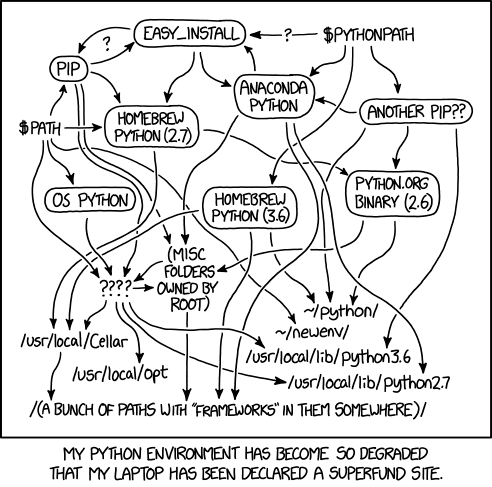
Python Environment Hell
From XKCD (Creative Commons Attribution-NonCommercial 2.5 License)
Let us have a look at how we can create and manage virtual environments from the command line
using venv and manage packages using pip.
Creating Virtual Environments Using venv
Creating a virtual environment with venv is done by executing the following command:
$ python3 -m venv /path/to/new/virtual/environment
where /path/to/new/virtual/environment is a path to a directory where you want to place it -
conventionally within your software project so they are co-located.
This will create the target directory for the virtual environment
(and any parent directories that don’t exist already).
For our project let’s create a virtual environment called “venv”. First, ensure you are within the project root directory, then:
$ python3 -m venv venv
If you list the contents of the newly created directory “venv”, on a Mac or Linux system (slightly different on Windows as explained below) you should see something like:
$ ls -l venv
total 8
drwxr-xr-x  12 alex  staff  384  5 Oct 11:47 bin
drwxr-xr-x   2 alex  staff   64  5 Oct 11:47 include
drwxr-xr-x   3 alex  staff   96  5 Oct 11:47 lib
-rw-r--r--   1 alex  staff   90  5 Oct 11:47 pyvenv.cfg
So, running the python3 -m venv venv command created the target directory called “venv”
containing:
pyvenv.cfgconfiguration file with a home key pointing to the Python installation from which the command was run,binsubdirectory (calledScriptson Windows) containing a symlink of the Python interpreter binary used to create the environment and the standard Python library,lib/pythonX.Y/site-packagessubdirectory (calledLib\site-packageson Windows) to contain its own independent set of installed Python packages isolated from other projects,- various other configuration and supporting files and subdirectories.
Naming Virtual Environments
What is a good name to use for a virtual environment? Using “venv” or “.venv” as the name for an environment and storing it within the project’s directory seems to be the recommended way - this way when you come across such a subdirectory within a software project, by convention you know it contains its virtual environment details. A slight downside is that all different virtual environments on your machine then use the same name and the current one is determined by the context of the path you are currently located in. A (non-conventional) alternative is to use your project name for the name of the virtual environment, with the downside that there is nothing to indicate that such a directory contains a virtual environment. In our case, we have settled to use the name “venv” instead of “.venv” since it is not a hidden directory and we want it to be displayed by the command line when listing directory contents (the “.” in its name that would, by convention, make it hidden). In the future, you will decide what naming convention works best for you. Here are some references for each of the naming conventions:
- The Hitchhiker’s Guide to Python notes that “venv” is the general convention used globally
- The Python Documentation indicates that “.venv” is common
- “venv” vs “.venv” discussion
Once you’ve created a virtual environment, you will need to activate it.
On Mac or Linux, it is done as:
$ source venv/bin/activate
(venv) $
On Windows, recall that we have Scripts directory instead of bin
and activating a virtual environment is done as:
$ source venv/Scripts/activate
(venv) $
Activating the virtual environment will change your command line’s prompt to show what virtual environment you are currently using (indicated by its name in round brackets at the start of the prompt), and modify the environment so that running Python will get you the particular version of Python configured in your virtual environment.
You can verify you are using your virtual environment’s version of Python
by checking the path using the command which:
(venv) $ which python3
/home/alex/InterPython_Workshop_Example/venv/bin/python3
When you’re done working on your project, you can exit the environment with:
(venv) $ deactivate
If you’ve just done the deactivate,
ensure you reactivate the environment ready for the next part:
$ source venv/bin/activate
(venv) $
Python Within A Virtual Environment
Within a virtual environment, commands
pythonandpipwill refer to the version of Python you created the environment with. If you create a virtual environment withpython3 -m venv venv,pythonwill refer topython3andpipwill refer topip3.On some machines with Python 2 installed,
pythoncommand may refer to the copy of Python 2 installed outside of the virtual environment instead, which can cause confusion. You can always check which version of Python you are using in your virtual environment with the commandwhich pythonto be absolutely sure. We continue usingpython3andpip3in this material to avoid confusion for those users, but commandspythonandpipmay work for you as expected.
Note that, since our software project is being tracked by Git, the newly created virtual environment will show up in version control - we will see how to handle it using Git in one of the subsequent episodes.
Installing External Packages Using pip
We noticed earlier that our code depends on two external packages/libraries -
pandas and matplotlib.
In order for the code to run on your machine,
you need to install these two dependencies into your virtual environment.
To install the latest version of a package with pip
you use pip’s install command and specify the package’s name, e.g.:
(venv) $ pip3 install pandas
(venv) $ pip3 install matplotlib
or like this to install multiple packages at once for short:
(venv) $ pip3 install pandas matplotlib
How About
python3 -m pip install?Why are we not using
pipas an argument topython3command, in the same way we did withvenv(i.e.python3 -m venv)?python3 -m pip installshould be used according to the official Pip documentation; other official documentation still seems to have a mixture of usages. Core Python developer Brett Cannon offers a more detailed explanation of edge cases when the two options may produce different results and recommendspython3 -m pip install. We kept the old-style command (pip3 install) as it seems more prevalent among developers at the moment - but it may be a convention that will soon change and certainly something you should consider.
If you run the pip3 install command on a package that is already installed,
pip will notice this and do nothing.
To install a specific version of a Python package
give the package name followed by == and the version number,
e.g. pip3 install pandas==2.1.2.
To specify a minimum version of a Python package,
you can do pip3 install pandas>=2.1.0.
To upgrade a package to the latest version, e.g. pip3 install --upgrade pandas.
To display information about a particular installed package do:
(venv) $ pip3 show pandas
Name: pandas
Version: 2.1.4
Summary: Powerful data structures for data analysis, time series, and statistics
Home-page: https://pandas.pydata.org
Author:
Author-email: The Pandas Development Team <pandas-dev@python.org>
License: BSD 3-Clause License
...
Requires: numpy, python-dateutil, pytz, tzdata
Required-by:
To list all packages installed with pip (in your current virtual environment):
(venv) $ pip3 list
Package         Version
--------------- -------
contourpy       1.2.0
cycler          0.12.1
fonttools       4.47.2
kiwisolver      1.4.5
matplotlib      3.8.2
numpy           1.26.3
packaging       23.2
pandas          2.1.4
pillow          10.2.0
pip             23.3.2
pyparsing       3.1.1
python-dateutil 2.8.2
pytz            2023.3.post1
setuptools      65.5.0
six             1.16.0
tzdata          2023.4
To uninstall a package installed in the virtual environment do: pip3 uninstall package-name.
You can also supply a list of packages to uninstall at the same time.
Exporting/Importing Virtual Environments Using pip
You are collaborating on a project with a team so, naturally,
you will want to share your environment with your collaborators
so they can easily ‘clone’ your software project with all of its dependencies
and everyone can replicate equivalent virtual environments on their machines.
pip has a handy way of exporting, saving and sharing virtual environments.
To export your active environment -
use pip3 freeze command to produce a list of packages installed in the virtual environment.
A common convention is to put this list in a requirements.txt file:
(venv) $ pip3 freeze > requirements.txt
(venv) $ cat requirements.txt
contourpy==1.2.0
cycler==0.12.1
fonttools==4.47.2
kiwisolver==1.4.5
matplotlib==3.8.2
numpy==1.26.3
packaging==23.2
pandas==2.1.4
pillow==10.2.0
pyparsing==3.1.1
python-dateutil==2.8.2
pytz==2023.3.post1
six==1.16.0
tzdata==2023.4
The first of the above commands will create a requirements.txt file in your current directory.
Yours may look a little different,
depending on the version of the packages you have installed,
as well as any differences in the packages that they themselves use.
The requirements.txt file can then be committed to a version control system
(we will see how to do this using Git in one of the following episodes)
and get shipped as part of your software and shared with collaborators and/or users.
They can then replicate your environment
and install all the necessary packages from the project root as follows:
(venv) $ pip3 install -r requirements.txt
As your project grows - you may need to update your environment for a variety of reasons.
For example, one of your project’s dependencies has just released a new version
(dependency version number update),
you need an additional package for data analysis (adding a new dependency)
or you have found a better package and no longer need the older package
(adding a new and removing an old dependency).
What you need to do in this case
(apart from installing the new and removing the packages that are no longer needed
from your virtual environment)
is update the contents of the requirements.txt file accordingly
by re-issuing pip freeze command
and propagate the updated requirements.txt file to your collaborators
via your code sharing platform (e.g. GitHub).
Official Documentation
For a full list of options and commands, consult the official
venvdocumentation and the Installing Python Modules withpipguide. Also check out the guide “Installing packages usingpipand virtual environments”.
Installing Jupyter Lab
Jupyter Lab itself comes as a Python package. Therefore, we have to install it
in the environment as well. Another package that we will need for our project is astropy,
which provides a lot of functions, useful for writing astronomical software and data processing.
(venv) $ pip3 install astropy
(venv) $ pip3 install jupyterlab
Do not forget to update the requirements.txt file after the installation is finished.
If you run pip freeze, you will see that Jupyter Lab installed a lot of dependencies libraries,
so the list of requirements is now much larger.
Key Points
Virtual environments keep Python versions and dependencies required by different projects separate.
A virtual environment is itself a directory structure.
Use
venvto create and manage Python virtual environments.Use
pipto install and manage Python external (third-party) libraries.
pipallows you to declare all dependencies for a project in a separate file (by convention calledrequirements.txt) which can be shared with collaborators/users and used to replicate a virtual environment.Use
pip3 freeze > requirements.txtto take snapshot of your project’s dependencies.Use
pip3 install -r requirements.txtto replicate someone else’s virtual environment on your machine from therequirements.txtfile.
Integrated Software Development Environments
Overview
Teaching: 25 min
Exercises: 15 minQuestions
What are Integrated Development Environments (IDEs)?
What are the advantages of using IDEs for software development?
How does Jupyter Lab interact with virtual environments?
Objectives
Set up Jupyter Lab and its kernels
Use Jupyter Lab to run a script
Introduction
As we have seen in the previous episode - even a simple software project is typically split into smaller functional units and modules, which are kept in separate files and subdirectories. As your code starts to grow and becomes more complex, it will involve many different files and various external libraries. You will need an application to help you manage all the complexities of, and provide you with some useful (visual) facilities for, the software development process. Such clever and useful graphical software development applications are called Integrated Development Environments (IDEs).
Integrated Development Environments
An IDE normally consists of at least a source code editor, build automation tools and a debugger. The boundaries between modern IDEs and other aspects of the broader software development process are often blurred. Nowadays IDEs also offer version control support, tools to construct graphical user interfaces (GUI) and web browser integration for web app development, source code inspection for dependencies and many other useful functionalities. The following is a list of the most commonly seen IDE features:
- syntax highlighting - to show the language constructs, keywords and the syntax errors with visually distinct colours and font effects
- code completion - to speed up programming by offering a set of possible (syntactically correct) code options
- code search - finding package, class, function and variable declarations, their usages and referencing
- version control support - to interact with source code repositories
- debugging - for setting breakpoints in the code editor, step-by-step execution of code and inspection of variables
IDEs are extremely useful and modern software development would be very hard without them. There are a number of IDEs available for Python development; a good overview is available from the Python Project Wiki. In addition to IDEs, there are also a number of code editors that have Python support. Code editors can be as simple as a text editor with syntax highlighting and code formatting capabilities (e.g., GNU EMACS, Vi/Vim). Most good code editors can also execute code and control a debugger, and some can also interact with a version control system. Compared to an IDE, a good dedicated code editor is usually smaller and quicker, but often less feature-rich. You will have to decide which one is the best for you - in this course, we will use Jupyter Lab - a free open-source web-based IDE familiar to most Python-coding astronomers.
Is Jupyter Lab an IDE?
For a long time, Jupyter Notebook was not considered as a full-fledged IDE. The main argument against considering Jupyter Notebooks an IDE was that it lacked a lot of functionality that is essential for the full cycle of software development. The most notable instrument that wasn’t present in Jupyter Notebook was the debugger.
However, modern versions of Jupyter Lab, an evolutionary development of Jupyter Notebook, come with the built-in debugger, as well as with all the rest of the basic IDE instruments. Formally, this makes Jupyter Lab a ‘real’ IDE. At the same time, Jupyter Lab and classic IDEs (such as PyCharm or Spyder) impose distinctly different coding routines. Jupyter Lab (as Jupyter Notebook before) assumes an interactive cell-by-cell development and execution of the code, which is well-suited for data exploration and analysis and for small-scale software development. At the same time, for larger projects that do not require executing small parts of the code separately, ‘classic’ IDEs are more suitable.
Using Jupyter Lab
Let’s open our project in Jupyter Lab now and familiarise ourselves with some commonly used features.
Jupyter Lab interface
To launch Jupyter Lab, activate the venv environment created in the previous episode and type in the terminal:
(venv) $ jupyter lab
The output will look similar to this:
 To access the server, open this file in a browser:
        file:///home/alex/.local/share/jupyter/runtime/jpserver-2946113-open.html
    Or copy and paste one of these URLs:
        http://localhost:8888/lab?token=e2aff7125e9917868a16b8b627f73995eb83effbcafeee05
        http://127.0.0.1:8888/lab?token=e2aff7125e9917868a16b8b627f73995eb83effbcafeee05
Now you can click on one of the URLs below and Jupyter Lab will open in your browser.
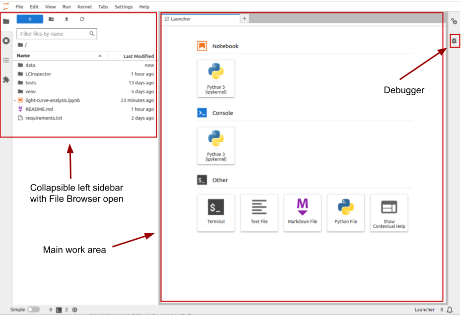
Jupyter Lab starting interface
The Jupyter Lab interface includes the following areas:
- Menu bar, from which you can access most common Jupyter Lab functions;
- A collapsible left sidebar, in which four tabs are present:
- File Manager. From here you can manage the files and directories in your repository folder.
- Running terminal and kernels. Here you can find the list of running Jupyter Notebook kernels and console sessions.
- Table of contents. Here Jupyter Lab will automatically generate a table of contents of your notebooks (using headers and other markdown cells) and Python files (using function and class definitions).
- Extension Manager. In this section, it is possible to install extensions that expand Jupyter Lab functionality, for example, allowing integration with Git, adding CSS formatting, and so on.
- The main work area. When you just opened Jupyter Lab, you can see several options for starting your work, such as creating a new Notebook, opening a new Python console session, or creating a new text or Python file. The list of these options will vary depending on which kernels and programming languages you have installed. When you open a Notebook or a file, it will appear in a separate tab in this area.
- In the right collapsible sidebar you can access the notebooks’ Properties Manager and Debugger, which can be used for inspecting the variables and managing Breakpoints.
Making Jupyter Lab show hidden files
By default, Jupyter Lab file manager does not show hidden files. If you prefer to change that, you need to enable a corresponding option in Jupyter Lab configuration file. In the terminal run:
$ jupyter --pathsconfig: /home/alex/.jupyter ... data: /home/alex/.local/share/jupyter ...This command lists the folders in which Jupyter will look for configuration files, ordered by precedence. In all likelyhood, you already have a config file called
jupyter_server_config.pyin the upmost folder:$ ls -l /home/alex/.jupytertotal 84 -rw-rw-r-- 1 alex alex 69714 Jul 1 12:38 jupyter_server_config.py drwxrwxr-x 4 alex alex 4096 Feb 4 14:28 lab ...If not, you can generate it by typing:
$ jupyter server --generate-configNext, open it with any text editor, for example:
$ gedit /home/alex/.jupyter/jupyter_server_config.pyand find
c.ContentsManager.allow_hiddenparameter. By default it is commented out and set toFalse, so you need to uncomment it and change its value toTrue, and then save the file.After that go to the Jupyter Lab window and choose
View > Show hidden files, and hidden files will be available through the Jupyter Lab file browser. It is handy when you need to edit some hidden configuration files or keep track on temporal files created by your code, and if you don’t need it for some particular project, you can always switch it off by uncheckingView > Show hidden files.
Opening a Software Project
In the left sidebar, open the File Browser and look through the files present here. You can inspect the requirements.txt file, where we saved the list
of packages installed in our virtual environment, and README.md, containing some basic information about the project. Later we will add more information to
this file. For now, double click on the light-curve-analysis.ipynb.
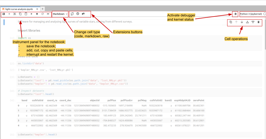
In the opened tab we can see a number of cells. Some of them contain Python code, while others display formatted text (‘Markdown’).
You can change the type of the cell in the drop-down menu in the instrumental panel on the top of the tab. You can execute cells
one by one by pressing Shift+Enter, or run them all by choosing Run > Run All in the main menu or by pressing a corresponding
button in the tab instrumental panel. Code cells produce outputs, which may contain text, tables and static or interactive plots.
Interface elements of a notebook tab
By default the notebooks are opened in tabs that take the full screen, however, you can align them vertially
or horizontally by dragging them in the preferred place. You can also place an output of any cell into a separate tab.
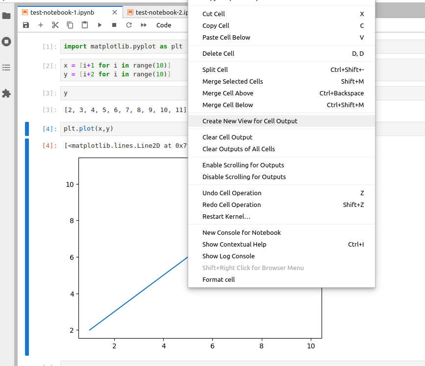
For this, make a right-click on
the output content and choose Create New View for Cell Output. You can open multiple tabs for the cell outputs and
reorder them in the same way as the notebook tabs.
Creating cell output view
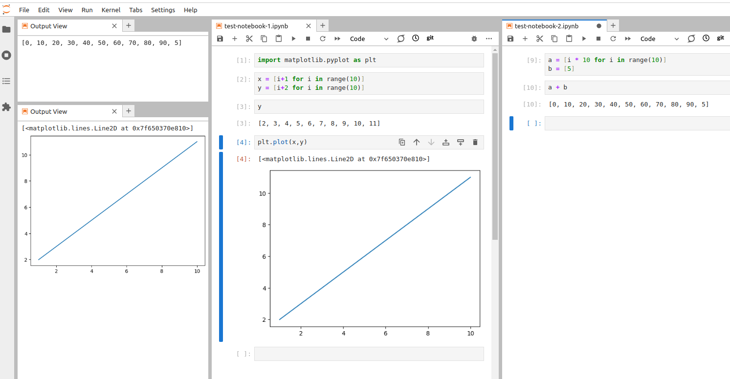
You can order the notebook tabs and cell output views any way you like
The code in the notebook is displayed using different colours, following the rules set up for
the syntax highlighting.
Syntax highlighting is a feature that displays source code terms
in different colours and fonts according to the syntax category the highlighted term belongs to.
It also makes syntax errors visually distinct.
Highlighting does not affect the meaning of the code itself -
it’s intended only for humans to make reading code and finding errors easier. The code highlighting
color scheme depends on the programming language (or, to be more precise,
on the kernel which is currently connected to your Notebook), and in the Text Editor, you can pick the language yourself
in View > Text Editor Syntax Highlighting menu.
By default it is inferred from the file extension, e.g. Python for .py files.
Code Completion & Documentation References
Context-aware code completion suggestions (`Tab`)
Contextual help in a pop-up window (`Shift+Tab`)
Setting up auto-completion
When you are typing code, you can use completion suggestions and contextual help tools, included in Jupyter Lab. You can use three hotkey combinations for using these tools:
- When you start typing a command, you can press
Tab, and Jupyter Lab will offer you options of code that can follow. - You also can type
Shift+Tabto open contextual help in a pop-up window. - Another option is to use
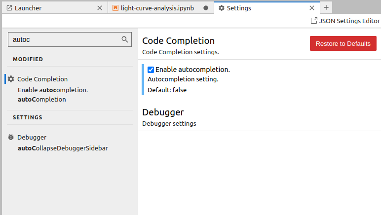
Ctrl+Ifor opening contextual help in the right sidebar. - Finally, you can enable code auto-completion. For this, go to ‘Settings > Settings Editor’ and start typing ‘auto-completion’ in the Search box. Then select the ‘Enable autocompletion’ checkbox.
Using context-aware code completion features speeds up the process of coding, and reduces typos and other common mistakes. Using contextual help also improves the quality of the code, as well as simplifies the process for the programmer.
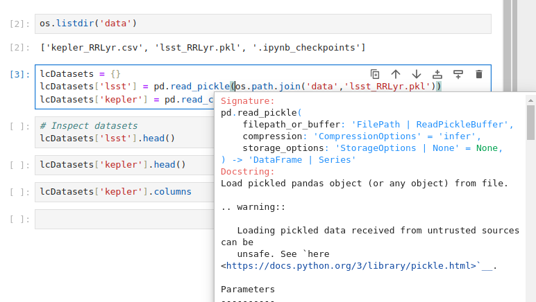
How does contextual help work?
Contextual help relies on the docstrings, written in the library’s source files by the developers. If you look at code definitions of well-maintained libraries, such as Pandas or Numpy, you will see that the docstrings are very detailed: they contain input parameters, outputs, algorithm descriptions, and even examples of usage. Later we will talk about how to write good docstrings, but here you can see why they are so essential.
Try completion, auto-completion, and contextual help functions
Execute already existing cells of the notebook. There are several ways to do this:
- You can go through the cells, clicking
Shift+Enteron each of them.- You can use
Run > Run all cellsmenu.- You can use
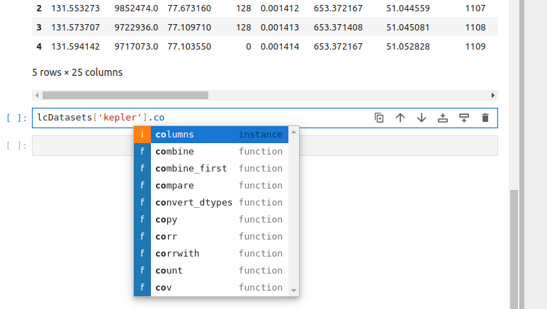
Restart the kernel and run all cellsbutton on the tool panel on the top of your notebook tab. Be aware that when you restart the kernel, you lose all the data from already executed code, e.g. all the variables will be deleted.After that, inspect contextual help of several functions, e.g.
pd.read_pickle,np.array, andos.path.join. Pay attention to which information is included in the contextual help and in which format. Next, get the list of the columns in one of the opened datasets, using completion at every step.Solution
To get the list of the columns you can use the following code:
LcDatasets['kepler'].columns. By pressingTabonce you started typing ‘LcDatasets’, ‘kepler’ and ‘columns’, you will get suggestions for the available options of the following code.After that, enable auto-completion and get the list of the columns of the second dataset. Depending on what is more convenient for you, you can leave auto-completion function turned on, or turn it off.
Code Search
Jupyter Lab offers you the possibility to search and replace text within the file, using case matching and regular expressions.
You can perform the search within the whole document or only in a single cell, with or without cell outputs (the results of execution
of the code within the cell). To access the search tool, use Ctrl+F key combination, or Edit > Find in the main menu.
Searching across multiple notebooks
Jupyter Lab built-in search does not allow searching strings across multiple files. However, such functionality is available with jupyterlab-search-replace extension.
Jupyter Lab magic
Jupyter magic commands or simply magics are special commands, provided by the default Jupyter kernel (‘backend’ that
executes the code) called IPython. Magics allow us to conveniently perform many useful operations since they can interact
with operational system and Jupyter kernels.
There are two types of magics: the ones that operate on a single line of the following code (the code has to be written on the same line
after a single space, without parenthesis or quotation marks), and the ones that act upon
the content of a whole single cell. The line magics are preceded by a single percentage symbol (%), while cell magics
use two percentage symbols (%%). Here is a short list of the most useful magics:
%magic: prints information about magics system%lsmagic: lists all magic commands in a convenient form%quickref: another helper function that shows references for the magic commands%time,%timeitand%%timeit: measure the execution time of the code.%cd,%ls,%pwdand other console commands: executes terminal commands%run: executes another ‘.ipynb’ or ‘.py’ file from within the current notebook%who: lists the defined variables. It is possible to list only variables of a certain type, e.g.%who string
%time,%timeitand%%timeitThe difference between
%timeand%timeitis that first command executes your code only once, while the second runs it several times and measures the average execution time, attempting to get a more precise value. However, the second command isn’t always better! For example, if you measure the execution time of a list sorting, after the first execution the list will already be sorted, and executing the same code over already sorted list will take much less time, meaning that the average execution time will be skewed towards lesser numbers.%%timeit, as follows from two ‘%’ signs, measures the execution time for all code in a cell together.
Try out different magics
Try several different magic commands, such as
%lsmagic,%pwdand%who. Use%whocommand to get the list ofdictvariables (pay attention, that if you use%whocommand without specifying the type of the variable, it will also include the packages that you imported in the notebook).
Apart from the built-in magics, there are many more that you can install additionally. It is also possible to develop your own magic commands.
Installing packages from Jupyter notebook interface or Jupyter console session
Since magics allow us to execute terminal commands, there is a way to install Python packages right from the Jupyter interface. We can run
%pip3 install astropyright in a Jupyter cell. This is a standard way of installing packages in cloud Jupyter Notebook services, such as Google Colab or the Notebook aspect of Rubin Science Platform. Pay attention, though, that another common way of doing this, using!instead of%before the installation command, is in general not safe and can lead to the dependencies issues due to the particularities of how OS and Jupyter kernels interact. You can still see it often, since magic command forpipappeared only in the later versions of IPython.
Key Points
An IDE is an application that provides a comprehensive set of facilities for software development, including syntax highlighting, code search and completion, version control, testing and debugging.
Jupyter Lab launches within the pre-existing virtual environment
We can run terminal commands within Jupyter Lab
Best practices for Jupyter
Overview
Teaching: 15 min
Exercises: 10 minQuestions
How to avoid chaos when writing code in Notebooks?
What is the workflow when using Jupyter Lab for software development?
Objectives
Follow best practice to ensure that your Notebook is well-organized and reusable.
Pros and Cons of Interactivity
Jupyter notebooks are very convenient since they allow executing pieces of code in an arbitrary order, giving the developer a high level of interactivity. The other side of the coin is that notebooks enable the development of the code without a clear structure, and that the result of the executed code differs depending on which cells were executed prior to that. Taking care of keeping the code in order falls on the developer’s shoulders even more than when a classic IDE is used.
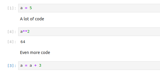
Inattention to cell execution order can mess your data
As a result, Jupyter Lab is not recommended for large-scale software development,
and even for smaller projects the final code should always be extracted into executable
‘.py’ files and converted into Python package. At the same time, notebooks are well-suited for
data inverstigation, visualization and presentations, and it is the best when .ipynb files
contain only the code related to those tasks. Even then, without following certain
best practices, notebooks have poor reproducibility.
Jupyter Lab best practices
Fortunately, Jupyter Lab provides us with a number of tools that allow us to keep the notebook files clean, and the developed code reliable. Let’s consider the most important rules of keeping your notebooks in a good condition:
- Set the objective. Define the objective of the notebook from the start and write it on the top of the notebook. Pay attention to how you phrase the objective: it should explain what is done in this notebook and be specific. E.g. instead of generic ‘Some code for analysing the data’ it is better to write ‘Inspect, clean from NaNs and visualize on a histogram LSST RR Lyrae light curves dataset’.
- One notebook - one task. One notebook should correspond to only one task or stage of your investigation. E.g. it is better to separate data preprocessing and visualization, or analysis of the spectra and analysis of the light curves. Do not stray from this objective; you definitely will get new ideas while working on your analysis, but if they are outside of the scope of this particular notebook, they should be extracted to a new file. There are two possible exceptions to this rule: if your notebook is really small (e.g. you just need to make a couple of plots), or if it’s a demonstration or presentation notebook.
- Structure first.Think about the structure of the notebook before you start working, and write the headers of the sections
in advance. For most astronomical projects, you will need at least four sections: imports, loading the data,
pre-processing the data and analysis itself. Remember, that you can create subsections using secondary headers!
It is also a good idea to put variables, that later will be used across the code (e.g. sizes of samples, time ranges for
period search, magnitude limits) into a separate section before the analysis, and create temporary sections for classes and functions
(which ultimately should be extracted into
.pyfiles). - Utilize Markdown cells for detailed explanations of what is done in the following code cells. Markdown cells
allow you to use headers, common types of text formatting, such as bold, italics and strikethrough formatting,
create lists, separators and tables, insert latex equations and use HTML formatting and so on. Here is a
cheat sheet for the
common types of formatting. To convert the cell into Markdown, you can press
Escand thenM, or by using the drop-down menu in the instrumental panel at the top of the notebook tab. -
Keep it short. Keep your notebooks short. There is no hard rule, but constraining a notebook to a hundred of cells is a good idea. If your notebook is longer than that, make sure that you follow the rule of ‘One notebook - one task’.
Jupyter Lab Table of Contents
The benefit of using multi-level headers for sections and subsections is that Jupyter Lab uses them for creating the Table of Contents, which can be accesses from the collapsible left side-bar. With this panel, you can quickly evaluate the structure of your notebook, go to any subsection or execute all the cells under the selected header.
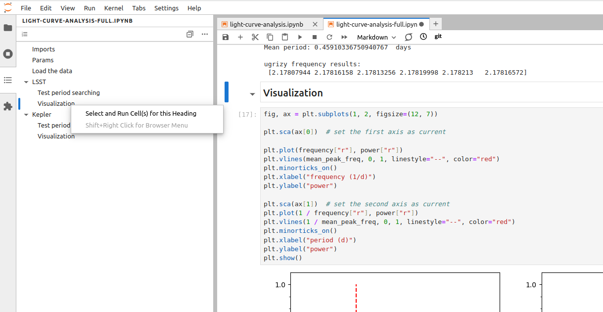
Using the Table of Contents to execute cells in a selected section
Fix the structure of the ‘light-curve-analysis.ipynb’ notebook
Go through the best practices listed above one by one and improve the structure of the
light-curve-analysis.ipynbnotebook.Solution
Let’s go through the recommendations one by one.
- Set the objective. Right now the objective of the notebook is phrased in a generic way. We can rephrase it into, e.g. ‘Inspect the sizes and visualize light curves from the LSST and Kepler RR Lyrae datasets.’
- One notebook - one task. Since for now our notebook is small, we can leave it as it is. However, potentially we could have put visualization into a separate notebook.
- Structure first. Currently the structure of the notebook is not well-defined. Add headers for the sections dedicated to the
inspection of the datasets and visialization of a light curve, put all imports into the corresponding section and move the variables
that we are likely to use in different sections to the ‘Params’ section
(in our case it can be
plot_filter_labels,plot_filter_colorsandplot_filter_symbols). - Keep it short. Since our notebook has less than a hundred cells, for now we don’t have this problem.
- Utilize Markdown cells. Give a brief description for each section (you can put it in the same cell as the headers). Use some formatting, e.g. in the ‘Dataset inspection’ section create a table listing the number of objects in current versions of each of the datasets.
What about the code that has to be executed only once, and then skipped?
Let’s say you have some code that has to be executed only once, and in the next executions of the notebook it has to be skipped. Such situations often arise during data pre-processing, when some data has to be downloaded or cleaned from NaNs only once, and in the subsequent executions of the notebook loaded from the saved copy. Taking these pieces of code into a separate notebook is not always convenient, and using comments to make this code inactive makes your notebook hard to understand in the future. A good way to handle such situations is to use boolean flags to indicate which steps have to be executed, and which should be skipped. By storing these flags in the ‘Parameters’ section you can quickly see the current state of your work, and turn on and off different steps of the data processing as needed.
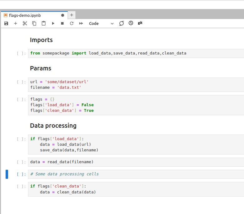
Using boolean flags to indicate parts of the code that has to be skipped
- Keep an eye on performance. If your notebook contains pieces of code that are computationally
expensive, work on a small representative sample of the data instead. When the code is ready, convert it into
an executable
.pyfile and launch it from terminal. It will help you to avoid situations when the result of a long computation is lost due to the IDE crash, and also it will make it possible to launch your analysis on the machines where Jupyter Lab is not available, e.g. on a remote server. - Reuse your code wisely. The code that you use more than once has to be turned into functions. This recommendation is applicable in all situations, not only when you use notebooks.
- Package your code. It is convenient to use Jupyter Lab for developing your code, however, once it is
ready and tested, you should extract your classes and functions into
.pyfiles and then turn it into a Python package. This allows you to use this code again across multiple notebooks, in other IDEs or from command line. In the next few days we will talk more about how to package your code. - Use ‘Restart and Run All’ often. Executing cells out of order is one of the main source of errors when developing code in Jupyter Lab. For this reason, make a habit of regularly using the ‘Restart and Run All’ button, that will restart your kernel, delete all stored variables and execute all cells in the top-down order. Always do it before saving the notebook and pushing it into a Git repository. This habit greatly improves the reproducibility of your notebooks.
'Restart and Run All' button helps you to ensure that your notebook is executed in the right order
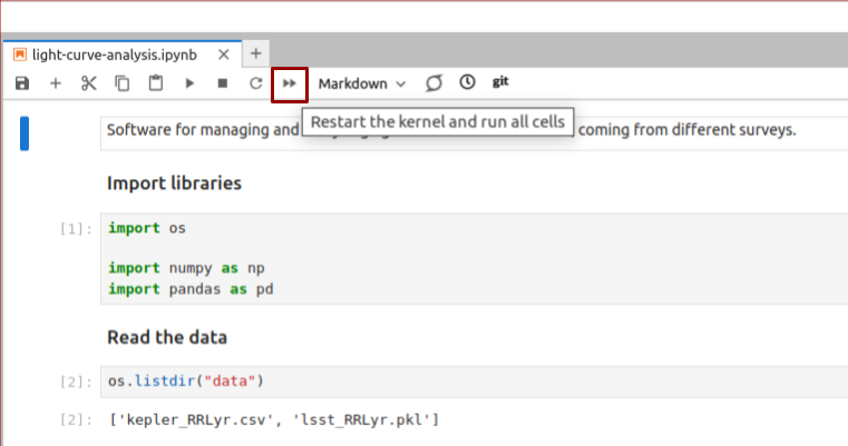
Shouldn’t We Clear Outputs of All Cells Before Pushing the Notebook into a Repo?
There is an old recommendation to always use
Restart Kernel and Clear Outputs of All Cellsbefore committing the notebook into a Git repository. This recommendation comes from the fact that native Git tools for comparing different versions of the files (git diff) do not handle.ipynbfiles well. Plots in the outputs are especially inconvenient, since they will show up as human-unreadable strings (which is what images are when you try to open them via text editor). However,git diffin general isn’t suitable for investigating changes in any files that are not, in essence, plain text. More so, clearing the outputs of the notebooks after you finished your work makes it impossible to e.g. use the notebook for a spontaneous presentation or demonstration of the results. The solution to this problem is to use the suitable instruments. Jupyter Lab has several extensions that allow to compare different versions of the notebooks, such asnbdimeandjupyterlab-git. More so, currently GitHub provides us with a possibility to use so called ‘Rich Jupyter Notebook Diffs’ when an updated notebook is pushed in your repository. You can enable this function by clicking on your avatar in the top right corner and then selectingFeature Preview > Rich Jupyter Notebook Diffs.
Jupyter Notebook, Rubin Science Platform and Google Colab
While RSP and Google Colab have Jupyter Notebook installed and not Jupyter Lab, all of the best practices above are still applicable on these platworms, with the only exception that you will have to create the Table of Contents manually.
Additional exercise
Open one of your recent notebooks and apply the best practices listed above to improve its structure. Do you need to reorder your code a lot? Is there some code that can be extracted into
.pyfiles?
Key Points
The interactivity of Notebooks, while convenient, enables chaotic style of software development.
We must follow best practices for Jupyter Lab to avoid chaos in the Notebooks.
Collaborative Software Development Using Git and GitHub
Overview
Teaching: 35 min
Exercises: 0 minQuestions
What are Git branches and why are they useful for code development?
What are some best practices when developing software collaboratively using Git?
Objectives
Commit changes in a software project to a local repository and publish them in a remote repository on GitHub
Create branches for managing different threads of code development
Learn to use feature branch workflow to effectively collaborate with a team on a software project
Introduction
So far we have checked out our software project from GitHub and used command line tools to configure a virtual environment for our project and run our code. We have also familiarised ourselves with Jupyter Lab - a graphical tool we will use for code development. We are now going to start using another set of tools from the collaborative code development toolbox - namely, the version control system Git and code sharing platform GitHub. These two will enable us to track changes to our code and share it with others.
You may recall that we have already made some changes to our project locally -
we created a virtual environment in the directory called “venv”
and exported it to the requirements.txt file.
We should now decide which of those changes we want to check in and share with others in our team.
This is a typical software development workflow -
you work locally on code,
test it to make sure it works correctly and as expected,
then record your changes using version control
and share your work with others via a shared and centrally backed-up repository.
Firstly, let’s remind ourselves how to work with Git from the command line.
Git Refresher
Git is a version control system for tracking changes in computer files and coordinating work on those files among multiple people. It is primarily used for source code management in software development but it can be used to track changes in files in general - it is particularly effective for tracking text-based files (e.g. source code files, CSV, Markdown, HTML, CSS, Tex, etc. files).
Git has several important characteristics:
- support for non-linear development allowing you and your colleagues to work on different parts of a project concurrently,
- support for distributed development allowing for multiple people to be working on the same project (even the same file) at the same time,
- every change recorded by Git remains part of the project history and can be retrieved at a later date, so even if you make a mistake you can revert to a point before it.
The diagram below shows a typical software development lifecycle with Git (starting from making changes locally) and the commonly used commands to interact with different parts of the Git infrastructure, such as:
- working directory -
a local directory (including any subdirectories) where your project files live
and where you are currently working.
It is also known as the “untracked” area of Git.
Any changes to files will be marked by Git in the working directory.
If you make changes to the working directory and do not explicitly tell Git to save them -
you will likely lose those changes.
Using
git add filenamecommand, you tell Git to start tracking changes to filefilenamewithin your working directory. - staging area (index) -
once you tell Git to start tracking changes to files
(with
git add filenamecommand), Git saves those changes in the staging area on your local machine. Each subsequent change to the same file needs to be followed by anothergit add filenamecommand to tell Git to update it in the staging area. To see what is in your working directory and staging area at any moment (i.e. what changes is Git tracking), run the commandgit status. - local repository -
stored within the
.gitdirectory of your project locally, this is where Git wraps together all your changes from the staging area and puts them using thegit commitcommand. Each commit is a new, permanent snapshot (checkpoint, record) of your project in time, which you can share or revert to. - remote repository -
this is a version of your project that is hosted somewhere on the Internet
(e.g., on GitHub, GitLab or somewhere else).
While your project is nicely version-controlled in your local repository,
and you have snapshots of its versions from the past,
if your machine crashes - you still may lose all your work. Furthermore, you cannot
share or collaborate on this local work with others easily.
Working with a remote repository involves pushing your local changes remotely
(using
git push) and pulling other people’s changes from a remote repository to your local copy (usinggit fetchorgit pull) to keep the two in sync in order to collaborate (with a bonus that your work also gets backed up to another machine). Note that a common best practice when collaborating with others on a shared repository is to always do agit pullbefore agit push, to ensure you have any latest changes before you push your own.

Software development lifecycle with Git
Checking-in Changes to Our Project
Let’s check-in the changes we have done to our project so far. The first thing to do upon navigating into our software project’s directory root is to check the current status of our local working directory and repository.
$ git status
On branch main
Your branch is up to date with 'origin/main'.

Untracked files:
  (use "git add <file>..." to include in what will be committed)
	requirements.txt
	venv/

nothing added to commit but untracked files present (use "git add" to track)
As expected,
Git is telling us that we have some untracked files -
requirements.txt and directory “venv” -
present in our working directory which we have not
staged nor committed to our local repository yet.
You do not want to commit the newly created directory “venv” and share it with others
because this directory is specific to your machine and setup only
(i.e. it contains local paths to libraries on your system
that most likely would not work on any other machine).
You do, however, want to share requirements.txt with your team
as this file can be used to replicate the virtual environment on your collaborators’ systems.
To tell Git to intentionally ignore and not track certain files and directories,
you need to specify them in the .gitignore text file in the project root.
Our project already has .gitignore,
but in cases where you do not have it -
you can simply create it yourself.
In our case, we want to tell Git to ignore the “venv” directory
(and “.venv” as another naming convention for directories containing virtual environments)
and stop notifying us about it.
Edit your .gitignore file in a text editor
and add a line containing “venv/” and another one containing “.venv/”.
It does not matter much in this case where within the file you add these lines,
so let’s do it at the end.
Your .gitignore should look something like this:
# IDEs
.vscode/
.idea/
.ipynb_checkpoints/

# Intermediate Coverage file
.coverage

# Output files
*.png

# Python runtime
*.pyc
*.egg-info
.pytest_cache

# Virtual environments
venv/
.venv/
You may notice that we are already not tracking certain files and directories
with useful comments about what exactly we are ignoring. For example, we
have .ipynb_checkpoints/, which stores your notebooks’ checkpoint files. When you
create a new repository with .ipynb notebooks, you’ll have to add this line in the
.gitignore yourself. You may also notice that each line in .gitignore is actually a pattern,
so you can ignore multiple files that match a pattern
(e.g. “*.png” will ignore all PNG files in the current directory).
If you run the git status command now,
you will notice that Git has cleverly understood that
you want to ignore changes to the “venv” directory so it is not warning us about it any more.
However, it has now detected a change to .gitignore file that needs to be committed.
$ git status
On branch main
Your branch is up to date with 'origin/main'.

Changes not staged for commit:
  (use "git add <file>..." to update what will be committed)
  (use "git restore <file>..." to discard changes in working directory)
	modified:   .gitignore

Untracked files:
  (use "git add <file>..." to include in what will be committed)
	requirements.txt

no changes added to commit (use "git add" and/or "git commit -a")
To commit the changes .gitignore and requirements.txt to the local repository,
we first have to add these files to staging area to prepare them for committing.
We can do that at the same time as:
$ git add .gitignore requirements.txt
Now we can commit them to the local repository with:
$ git commit -m "Add requirements.txt. Ignore venv folders."
Remember to use meaningful messages for your commits.
So far we have been working in isolation -
all the changes we have done are still only stored locally on our individual machines.
In order to share our work with others,
we should push our changes to the remote repository on GitHub.
Before we push our changes however, we should first do a git pull.
This is considered best practice, since any changes made to the repository -
notably by other people -
may impact the changes we are about to push.
This could occur, for example,
by two collaborators making different changes to the same lines in a file.
By pulling first, we are made aware of any changes made by others,
in particular if there are any conflicts between their changes and ours.
$ git pull
Now we’ve ensured our repository is synchronised with the remote one, we can now push our changes. Some time ago GitHub strengthened authentication requirements for Git operations accessing GitHub from the command line over HTTPS. This means you cannot use passwords for authentication over HTTPS any more - you either need to set up and use a personal access token for additional security if you want to continue to use HTTPS, or switch to use private and public key pair over SSH before you can push remotely the changes you made locally. So, when you run the command below:
$ git push origin main
Authentication Errors
If you get a warning that HTTPS access is deprecated, or a token is required, then you accidentally cloned the repository using HTTPS and not SSH. You can fix this from the command line by resetting the remote repository URL setting on your local repo:
$ git remote set-url origin git@github.com:<YOUR_GITHUB_USERNAME>/InterPython_Workshop_Example.git
In the above command,
origin is an alias for the remote repository you used when cloning the project locally
(it is called that by convention and set up automatically by Git
when you run git clone remote_url command to replicate a remote repository locally);
main is the name of our main (and currently only) development branch.
Git Remotes
Note that systems like Git allow us to synchronise work between any two or more copies of the same repository - the ones that are not located on your machine are “Git remotes” for you. In practice, though, it is easiest to agree with your collaborators to use one copy as a central hub (such as GitHub or GitLab), where everyone pushes their changes to. This also avoid risks associated with keeping the “central copy” on someone’s laptop. You can have more than one remote configured for your local repository, each of which generally is either read-only or read/write for you. Collaborating with others involves managing these remote repositories and pushing and pulling information to and from them when you need to share work.
Git - distributed version control system
From W3Docs (freely available)
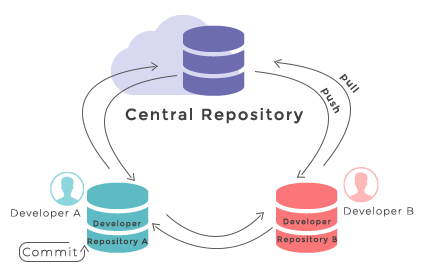
Git Branches
When we do git status,
Git also tells us that we are currently on the main branch of the project.
A branch is one version of your project (the files in your repository)
that can contain its own set of commits.
We can create a new branch,
make changes to the code which we then commit to the branch,
and, once we are happy with those changes,
merge them back to the main branch.
To see what other branches are available, do:
$ git branch
* main
At the moment, there’s only one branch (main)
and hence only one version of the code available.
When you create a Git repository for the first time,
by default you only get one version (i.e. branch) - main.
Let’s have a look at why having different branches might be useful.
Feature Branch Software Development Workflow
While it is technically OK to commit your changes directly to main branch,
and you may often find yourself doing so for some minor changes,
the best practice is to use a new branch for each separate and self-contained unit/piece of work
you want to add to the project.
This unit of work is also often called a feature
and the branch where you develop it is called a feature branch.
Each feature branch should have its own meaningful name -
indicating its purpose (e.g. “issue23-fix”).
If we keep making changes and pushing them directly to main branch on GitHub,
then anyone who downloads our software from there will get all of our work in progress -
whether or not it’s ready to use!
So, working on a separate branch for each feature you are adding is good for several reasons:
- it enables the main branch to remain stable while you and the team explore and test the new code on a feature branch,
- it enables you to keep the untested and not-yet-functional feature branch code under version control and backed up,
- you and other team members may work on several features at the same time independently from one another,
- if you decide that the feature is not working or is no longer needed - you can easily and safely discard that branch without affecting the rest of the code.
Branches are commonly used as part of a feature-branch workflow, shown in the diagram below.

Git feature branches
Adapted from Git Tutorial by sillevl (Creative Commons Attribution 4.0 International License)
In the software development workflow,
we typically have a main branch which is the version of the code that is
tested, stable and reliable.
Then, we normally have a development branch
(called develop or dev by convention)
that we use for work-in-progress code.
As we work on adding new features to the code,
we create new feature branches that first get merged into develop
after a thorough testing process.
After even more testing - develop branch will get merged into main.
The points when feature branches are merged to develop,
and develop to main
depend entirely on the practice/strategy established in the team.
For example, for smaller projects
(e.g. if you are working alone on a project or in a very small team),
feature branches sometimes get directly merged into main upon testing,
skipping the develop branch step.
In other projects,
the merge into main happens only at the point of making a new software release.
Whichever is the case for you, a good rule of thumb is -
nothing that is broken should be in main.
Creating Branches
Let’s create a develop branch to work on:
$ git branch develop
This command does not give any output,
but if we run git branch again,
without giving it a new branch name, we can see the list of branches we have -
including the new one we have just made.
$ git branch
    develop
  * main
The * indicates the currently active branch.
So how do we switch to our new branch?
We use the git checkout command with the name of the branch:
$ git checkout develop
Switched to branch 'develop'
Create and Switch to Branch Shortcut
A shortcut to create a new branch and immediately switch to it:
$ git checkout -b develop
Updating Branches
If we start updating and committing files now,
the commits will happen on the develop branch
and will not affect the version of the code in main.
We add and commit things to develop branch in the same way as we do to main.
Let’s make a small modification to lcanalyzer/models.py in Jupyter Lab,
and, say, add periods at the end of the docstrings for functions
mean_mag(),
max_mag() and
min_mag().
If we do:
$ git status
   On branch develop
   Changes not staged for commit:
     (use "git add <file>..." to update what will be committed)
     (use "git checkout -- <file>..." to discard changes in working directory)

   	modified:   lcanalyzer/models.py

   no changes added to commit (use "git add" and/or "git commit -a")
Git is telling us that we are on branch develop
and which tracked files have been modified in our working directory.
We can now add and commit the changes in the usual way.
$ git add lcanalyzer/models.py
$ git commit -m "Spelling fix"
Currently Active Branch
Remember,
addandcommitcommands always act on the currently active branch. You have to be careful and aware of which branch you are working with at any given moment.git statuscan help with that, and you will find yourself invoking it very often.
Pushing New Branch Remotely
We push the contents of the develop branch to GitHub
in the same way as we pushed the main branch.
However, as we have just created this branch locally,
it still does not exist in our remote repository.
You can check that in GitHub by listing all branches.
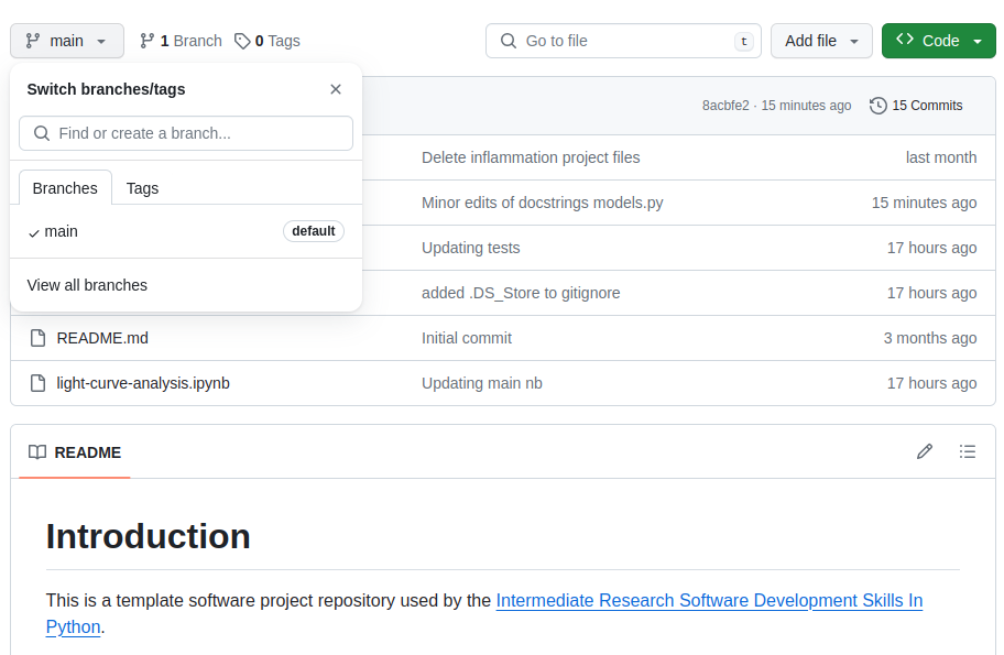
To push a new local branch remotely for the first time,
you could use the -u switch and the name of the branch you are creating and pushing to:
$ git push -u origin develop
Git Push With
-uSwitchUsing the
-uswitch with thegit pushcommand is a handy shortcut for: (1) creating the new remote branch and (2) setting your local branch to automatically track the remote one at the same time. You need to use the-uswitch only once to set up that association between your branch and the remote one explicitly. After that you could simply usegit pushwithout specifying the remote repository, if you wished so. We still prefer to explicitly state this information in commands.
Let’s confirm that the new branch develop now exist remotely on GitHub too.
From the < > Code tab in your repository in GitHub,
click the branch dropdown menu (currently showing the default branch main).
You should see your develop branch in the list too. Now the others can check out the develop branch too and continue to develop code on it.
After the initial push of the new branch,
each next time we push to it in the usual manner (i.e. without the -u switch):
$ git push origin develop
What is the Relationship Between Originating and New Branches?
It’s natural to think that new branches have a parent/child relationship with their originating branch, but in actual Git terms, branches themselves do not have parents but single commits do. Any commit can have zero parents (a root, or initial, commit), one parent (a regular commit), or multiple parents (a merge commit), and using this structure, we can build a ‘view’ of branches from a set of commits and their relationships. A common way to look at it is that Git branches are really only lightweight, movable pointers to commits. So as a new commit is added to a branch, the branch pointer is moved to the new commit.
What this means is that when you accomplish a merge between two branches, Git is able to determine the common ‘commit ancestor’ through the commits in a ‘branch’, and use that common ancestor to determine which commits need to be merged onto the destination branch. It also means that, in theory, you could merge any branch with any other at any time… although it may not make sense to do so!
Merging Into Main Branch
Once you have tested your changes on the develop branch,
you will want to merge them onto the main branch.
To do so, make sure you have all your changes committed and switch to main:
$ git checkout main
Switched to branch 'main'
Your branch is up to date with 'origin/main'.
To merge the develop branch on top of main do:
$ git merge develop
Updating 05e1ffb..be60389
Fast-forward
 lcanalyzer/models.py | 6 +++---
 1 files changed, 3 insertions(+), 3 deletions(-)
If there are no conflicts,
Git will merge the branches without complaining
and replay all commits from develop on top of the last commit from main.
If there are merge conflicts
(e.g. a team collaborator modified the same portion of the same file you are working on
and checked in their changes before you),
the particular files with conflicts will be marked
and you will need to resolve those conflicts
and commit the changes before attempting to merge again.
Since we have no conflicts, we can now push the main branch to the remote repository:
git push origin main
All Branches Are Equal
In Git, all branches are equal - there is nothing special about the
mainbranch. It is called that by convention and is created by default, but it can also be called something else. A good example isgh-pagesbranch which is often the source branch for website projects hosted on GitHub (rather thanmain).
Keeping Main Branch Stable
Good software development practice is to keep the
mainbranch stable while you and the team develop and test new functionalities on feature branches (which can be done in parallel and independently by different team members). The next step is to merge feature branches onto thedevelopbranch, where more testing can occur to verify that the new features work well with the rest of the code (and not just in isolation). We talk more about different types of code testing in one of the following episodes.
Practice branching without a repository
Understanding how git navigates branches and commits can be tricky. You can use an interactive visual simulator to master most of the common tasks, such as switching between branches, reverting your repository to the earlier state, browsing the history of a single file and so on, and get a better understanding of git under the hood.
Key Points
A branch is one version of your project that can contain its own set of commits.
Feature branches enable us to develop / explore / test new code features without affecting the stable
maincode.
Python Code Style Conventions
Overview
Teaching: 20 min
Exercises: 15 minQuestions
Why should you follow software code style conventions?
Who is setting code style conventions?
What code style conventions exist for Python?
Objectives
Understand the benefits of following community coding conventions
Introduction
We now have all the tools we need for software development and are raring to go. But before you dive into writing some more code and sharing it with others, ask yourself what kind of code should you be writing and publishing? It may be worth spending some time learning a bit about Python coding style conventions to make sure that your code is consistently formatted and readable by yourself and others.
“Any fool can write code that a computer can understand. Good programmers write code that humans can understand.” - Martin Fowler, British software engineer, author and international speaker on software development
Python Coding Style Guide
One of the most important things we can do to make sure our code is readable by others (and ourselves a few months down the line) is to make sure that it is descriptive, cleanly and consistently formatted and uses sensible, descriptive names for variable, function and module names. In order to help us format our code, we generally follow guidelines known as a style guide. A style guide is a set of conventions that we agree upon with our colleagues or community, to ensure that everyone contributing to the same project is producing code which looks similar in style. While a group of developers may choose to write and agree upon a new style guide unique to each project, in practice many programming languages have a single style guide which is adopted almost universally by the communities around the world. In Python, although we do have a choice of style guides available, the PEP 8 style guide is most commonly used. PEP here stands for Python Enhancement Proposals; PEPs are design documents for the Python community, typically specifications or conventions for how to do something in Python, a description of a new feature in Python, etc.
Style consistency
One of the key insights from Guido van Rossum, one of the PEP 8 authors, is that code is read much more often than it is written. Style guidelines are intended to improve the readability of code and make it consistent across the wide spectrum of Python code. Consistency with the style guide is important. Consistency within a project is more important. Consistency within one module or function is the most important. However, know when to be inconsistent - sometimes style guide recommendations are just not applicable. When in doubt, use your best judgment. Look at other examples and decide what looks best. And don’t hesitate to ask!
As we have already covered in the episode on Jupyter Lab IDE, Jupyter Lab highlights the language constructs (reserved words) and syntax errors to help us with coding.
A full list of style guidelines for this style is available from the PEP 8 website; here we highlight a few.
Indentation
Python is a kind of language that uses indentation as a way of grouping statements that belong to a particular block of code. Spaces are the recommended indentation method in Python code. The guideline is to use 4 spaces per indentation level - so 4 spaces on level one, 8 spaces on level two and so on. Many people prefer the use of tabs to spaces to indent the code for many reasons (e.g. additional typing, easy to introduce an error by missing a single space character, accessibility for individuals using screen readers, etc.) and do not follow this guideline. Whether you decide to follow this guideline or not, be consistent and follow the style already used in the project.
Indentation in Python 2 vs Python 3
Python 2 allowed code indented with a mixture of tabs and spaces. Python 3 disallows mixing the use of tabs and spaces for indentation. Whichever you choose, be consistent throughout the project.
Jupyter Lab has built-in support for converting tab indentation to spaces
for Python code in order to conform to PEP8.
So, you can type a tab character and Jupyter Lab will automatically convert it to 4 spaces.
For text files, in the Text Editor you can also control the amount of spaces that Jupyter Lab uses
to replace one tab character (Settings>Text Editor Indentation).
There are more complex rules on indenting single units of code that continue over several lines,
e.g. function, list or dictionary definitions can all take more than one line.
The preferred way of wrapping such long lines is
by using Python’s implied line continuation inside delimiters such as
parentheses (()),
brackets ([])
and braces ({}),
or a hanging indent.
# Add an extra level of indentation (extra 4 spaces) to distinguish arguments from the rest of the code that follows
def long_function_name(
        var_one, var_two, var_three,
        var_four):
    print(var_one)


# Aligned with opening delimiter
foo = long_function_name(var_one, var_two,
                         var_three, var_four)

# Use hanging indents to add an indentation level like paragraphs of text where all the lines in a paragraph are
# indented except the first one
foo = long_function_name(
    var_one, var_two,
    var_three, var_four)

# Using hanging indent again, but closing bracket aligned with the first non-blank character of the previous line
a_long_list = [
    [[1, 2, 3], [4, 5, 6], [7, 8, 9]], [[0.33, 0.66, 1], [0.66, 0.83, 1], [0.77, 0.88, 1]]
    ]

# Using hanging indent again, but closing bracket aligned with the start of the multiline contruct
a_long_list2 = [
    1,
    2,
    3,
    # ...
    79
]
More details on good and bad practices for continuation lines can be found in PEP 8 guideline on indentation.
Maximum Line Length
All lines should be up to 80 characters long;
for lines containing comments or docstrings (to be covered later)
the line length limit should be 73 -
see this discussion
for reasoning behind these numbers.
Some teams strongly prefer a longer line length,
and seemed to have settled on the length of 100.
Long lines of code can be broken over multiple lines
by wrapping expressions in delimiters,
as mentioned above (preferred method),
or using a backslash (\) at the end of the line
to indicate line continuation (slightly less preferred method).
# Using delimiters ( ) to wrap a multi-line expression
if (a == True and
    b == False):

# Using a backslash (\) for line continuation
if a == True and \
    b == False:
Should a Line Break Before or After a Binary Operator?
Lines should break before binary operators so that the operators do not get scattered across different columns on the screen. In the example below, the eye does not have to do the extra work to tell which items are added and which are subtracted:
# PEP 8 compliant - easy to match operators with operands
income = (gross_wages
          + taxable_interest
          + (dividends - qualified_dividends)
          - ira_deduction
          - student_loan_interest)
Blank Lines
Top-level function and class definitions should be surrounded with two blank lines. Method definitions inside a class should be surrounded by a single blank line. You can use blank lines in functions, sparingly, to indicate logical sections.
Whitespace in Expressions and Statements
Avoid extraneous whitespace in the following situations:
- immediately inside parentheses, brackets or braces
# PEP 8 compliant: my_function(colour[1], {id: 2}) # Not PEP 8 compliant: my_function( colour[ 1 ], { id: 2 } ) - Immediately before a comma,
semicolon,
or colon
(unless doing slicing where the colon acts like a binary operator
in which case it should should have equal amounts of whitespace on either side)
# PEP 8 compliant: if x == 4: print(x, y); x, y = y, x # Not PEP 8 compliant: if x == 4 : print(x , y); x , y = y, x - Immediately before the open parenthesis that starts the argument list of a function call
# PEP 8 compliant: my_function(1) # Not PEP 8 compliant: my_function (1) - Immediately before the open parenthesis that starts an indexing or slicing
# PEP 8 compliant: my_dct['key'] = my_lst[id] first_char = my_str[:, 1] # Not PEP 8 compliant: my_dct ['key'] = my_lst [id] first_char = my_str [:, 1] - More than one space around an assignment (or other) operator to align it with another
# PEP 8 compliant: x = 1 y = 2 student_loan_interest = 3 # Not PEP 8 compliant: x = 1 y = 2 student_loan_interest = 3 - Avoid trailing whitespace anywhere - it is not necessary and can cause errors.
For example, if you use backslash (
\) for continuation lines and have a space after it, the continuation line will not be interpreted correctly. - Surround these binary operators with a single space on either side: assignment (=), augmented assignment (+=, -= etc.), comparisons (==, <, >, !=, <>, <=, >=, in, not in, is, is not), booleans (and, or, not).
- Don’t use spaces around the = sign
when used to indicate a keyword argument assignment
or to indicate a default value for an unannotated function parameter
  # PEP 8 compliant use of spaces around = for variable assignment
  axis = 'x'
  angle = 90
  size = 450
  name = 'my_graph'

  # PEP 8 compliant use of no spaces around = for keyword argument assignment in a function call
  my_function(
      1,
      2,
      axis=axis,
      angle=angle,
      size=size,
      name=name)
String Quotes
In Python, single-quoted strings and double-quoted strings are the same. PEP8 does not make a recommendation for this apart from picking one rule and consistently sticking to it. When a string contains single or double quote characters, use the other one to avoid backslashes in the string as it improves readability.
Naming Conventions
There are a lot of different naming styles in use, including:
- lower_case_with_underscores (or snake_case)
- UPPER_CASE_WITH_UNDERSCORES
- CapitalisedWords (or PascalCase) (note: when using acronyms in CapitalisedWords, capitalise all the letters of the acronym, e.g HTTPServerError)
- camelCase (differs from CapitalisedWords/PascalCase by the initial lowercase character)
- Capitalised_Words_With_Underscores
As with other style guide recommendations - consistency is key. Follow the one already established in the project, if there is one. If there isn’t, follow any standard language style (such as PEP8 for Python). Failing that, just pick one, document it and stick to it.
Some things to be wary of when naming things in the code:
- Avoid any names that could cause confusion (e.g. lower case
lis hard to distinguish from a1(one), ‘O’ (uppercase o) from a ‘0’ (zero), ‘I’ (uppercase i) from ‘l’ (lowercase L)). - Avoid using non-ASCII (e.g. Unicode) characters for identifiers as these can trip up software that does not support Unicode.
- If your audience is international and English is the common language, try to use English words for identifiers and comments whenever possible but try to avoid abbreviations/local slang as they may not be understood by everyone. Also consider sticking with either ‘American’ or ‘British’ English spellings and try not to mix the two.
Function, Variable, Class, Module, Package Naming in Python
- Function and variable names should use lower_case_with_underscores
- Avoid single character names in almost all instances.
- Variable names should tell you what they store, and not just the type (e.g.
source_idis better thanstring)- Function names should tell you what the function does.
- Class names should use the CapitalisedWords convention.
- Modules should have short, all-lowercase names. Underscores can be used in the module name if it improves readability.
- Packages should also have short, all-lowercase names, although the use of underscores is discouraged.
A more detailed guide on naming functions, modules, classes and variables is available from PEP8.
Comments
Comments allow us to provide the reader with additional information on what the code does - reading and understanding source code is slow, laborious and can lead to misinterpretation, plus it is always a good idea to keep others in mind when writing code. A good rule of thumb is to assume that someone will always read your code at a later date, and this includes a future version of yourself. It can be easy to forget why you did something a particular way in six months’ time. Write comments as complete sentences and in English unless you are 100% sure the code will never be read by people who don’t speak your language.
The Good, the Bad, and the Ugly Comments
As a side reading, check out the ‘Putting comments in code: the good, the bad, and the ugly’ blogpost. Remember - a comment should answer the ‘why’ question”. Occasionally the “what” question. The “how” question should be answered by the code itself.
Block comments generally apply to some (or all) code that follows them,
and are indented to the same level as that code.
Each line of a block comment starts with a # and a single space
(unless it is indented text inside the comment).
def fahr_to_cels(fahr):
    # Block comment example: convert temperature in Fahrenheit to Celsius
    cels = (fahr + 32) * (5 / 9)
    return cels
An inline comment is a comment on the same line as a statement.
Inline comments should be separated by at least two spaces from the statement.
They should start with a # and a single space and should be used sparingly.
def fahr_to_cels(fahr):
    cels = (fahr + 32) * (5 / 9)  # Inline comment example: convert temperature in Fahrenheit to Celsius
    return cels
Python doesn’t have any multi-line comments, like you may have seen in other languages like C++ or Java. However, there are ways to do it using docstrings as we’ll see in a moment.
The reader should be able to understand a single function or method from its code and its comments, and should not have to look elsewhere in the code for clarification. The kind of things that need to be commented are:
- Why certain design or implementation decisions were adopted, especially in cases where the decision may seem counter-intuitive
- The names of any algorithms or design patterns that have been implemented
- The expected format of input files or database schemas
However, there are some restrictions. Comments that simply restate what the code does are redundant, and comments must be accurate and updated with the code, because an incorrect comment causes more confusion than no comment at all.
Exercise: Improve Code Style of Our Project
Let’s look at improving the coding style of our project. First create a new feature branch called
style-fixesoff ourdevelopbranch and switch to it (from the project root):$ git checkout develop $ git checkout -b style-fixesNext look at the
light-curve-analysis.ipynbfile and identify where the above guidelines have not been followed. Fix the discovered inconsistencies and commit them to the feature branch.Solution
There are a few things to fix in
light-curve-analysis.ipynb, for example:
Variable ‘LcDatasets’ uses CapitalisedWords naming convention which is recommended for class names but not variable names. By convention, variable names should be in lowercase with optional underscores so you should rename the variable ‘LcDatasets’ to, ‘lc_datasets’.
There is an extra blank line in cell 7, between the definition of ‘plot_filter_labels’ and ‘plot_filter_colors’. Normally, you should not use blank lines in the middle of the code unless you want to separate logical units - in which case only one blank line is used.
Line 3 in cell 7 (‘plot_filter_colors’ variable definition) is too long. A better style would be to use multiple lines and hanging indent, with the closing brace `}’ aligned either with the first non-whitespace character of the last line of list or the first character of the line that starts the multiline construct or simply moved to the end of the previous line. All three acceptable modifications are shown below.
 # Using hanging indent, with the closing '}' aligned with the first non-blank character of the previous line
plot_filter_colors = {
    "u": "#56b4e9",
    "g": "#008060",
    "r": "#ff4000",
    "i": "#850000",
    "z": "#6600cc",
    "y": "#000000",
    }
# Using hanging indent with the, closing '}' aligned with the start of the multiline contruct plot_filter_colors = { "u": "#56b4e9", "g": "#008060", "r": "#ff4000", "i": "#850000", "z": "#6600cc", "y": "#000000", }# Using hanging indent where all the lines of the multiline contruct are indented except the first one >> plot_filter_colors = { "u": "#56b4e9", "g": "#008060", "r": "#ff4000", "i": "#850000", "z": "#6600cc", "y": "#000000",}There are more style issues, but we will leave them for now to show how style fixes can be done automatically. Now, let’s add and commit our changes to the feature branch. We will check the status of our working directory first.
$ git statusOn branch style-fixes Changes not staged for commit: (use "git add <file>..." to update what will be committed) (use "git restore <file>..." to discard changes in working directory) modified: light-curve-analysis.ipynb no changes added to commit (use "git add" and/or "git commit -a")Git tells us we are on branch
style-fixesand that we have unstaged and uncommited changes tolight-curve-analysis.ipynb. Let’s commit them to the local repository.$ git add light-curve-analysis.ipynb $ git commit -m "Code style fixes."
Optional Exercise: Improve Code Style of Your Other Python Projects
If you have another Python project, check to which extent it conforms to PEP8 coding style.
Documentation Strings aka Docstrings
If the first thing in a function is a string that is not assigned to a variable, that string is attached to the function as its documentation. Consider the following code implementing function for calculating the nth Fibonacci number:
def fibonacci(n):
    """Calculate the nth Fibonacci number.

    A recursive implementation of Fibonacci array elements.

    :param n: integer
    :raises ValueError: raised if n is less than zero
    :returns: Fibonacci number
    """
    if n < 0:
        raise ValueError('Fibonacci is not defined for N < 0')
    if n == 0:
        return 0
    if n == 1:
        return 1

    return fibonacci(n - 1) + fibonacci(n - 2)
Note here we are explicitly documenting our input variables,
what is returned by the function,
and also when the ValueError exception is raised.
Along with a helpful description of what the function does,
this information can act as a contract for readers to understand what to expect in terms of
behaviour when using the function,
as well as how to use it.
A special comment string like this is called a docstring.
We do not need to use triple quotes when writing one,
but if we do, we can break the text across multiple lines.
Docstrings can also be used at the start of a Python module
(a file containing a number of Python functions)
or at the start of a Python class
(containing a number of methods)
to list their contents as a reference.
You should not confuse docstrings with comments though -
docstrings are context-dependent and should only be used in specific locations
(e.g. at the top of a module and immediately after class and def keywords as mentioned).
Using triple quoted strings in locations where
they will not be interpreted as docstrings
or using triple quotes as a way to ‘quickly’ comment out an entire block of code
is considered bad practice.
In our example case, we used the
Sphynx/ReadTheDocs docstring style
formatting for the param, raises and returns - other docstring formats exist as well.
Python PEP 257 - Recommendations for Docstrings
PEP 257 is another one of Python Enhancement Proposals and this one deals with docstring conventions to standardise how they are used. For example, on the subject of module-level docstrings, PEP 257 says:
The docstring for a module should generally list
the classes,
exceptions
and functions
(and any other objects)
that are exported by the module, with a one-line summary of each.
(These summaries generally give less detail than the summary line in the object's docstring.)
The docstring for a package
(i.e., the docstring of the package's `__init__.py` module)
should also list the modules and subpackages exported by the package.
Note that
__init__.pyfile used to be a required part of a package (pre Python 3.3) where a package was typically implemented as a directory containing an__init__.pyfile which got implicitly executed when a package was imported.
So, at the beginning of a module file we can just add
a docstring explaining the nature of a module.
For example, if fibonacci() was included in a module with other functions,
our module could have at the start of it:
"""A module for generating numerical sequences of numbers that occur in nature.

Functions:
  fibonacci - returns the Fibonacci number for a given integer
  golden_ratio - returns the golden ratio number to a given Fibonacci iteration
  ...
"""
...
The docstring for a function or a module
is returned when calling the help function and passing its name -
for example from the interactive Python console/terminal available from the command line
or when rendering code documentation online
(e.g. see Python documentation).
Jupyter Lab also displays the docstring for a function/module
in a little help popup window when using tab-completion or by pressing Ctrl+I.
help(fibonacci)
Exercise: Fix the Docstrings
Look into
models.pyin Jupyter Lab and improve docstrings for functionsmean_magandmax_magCommit those changes to feature branchstyle-fixes.Solution
For example, the improved docstrings for the above functions would contain explanations for parameters and return values.
def mean_mag(data,mag_col):
    """Calculate the mean magnitude of a lightcurve
    :param data: pd.DataFrame with observed magnitudes for a single source.
    :param mag_col: a string with the name of the column for calculating the mean.
    :returns: A float with mean value of the column
    """
    return np.mean(data[mag_col], axis=0)
def max_mag(data,mag_col): """Calculate the max magnitude of a lightcurve :param data: pd.DataFrame with observed magnitudes for a single source. :param mag_col: a string with the name of the column for calculating the max value. :returns: The max value of the column. """ return data[mag_col].max()Once we are happy with modifications, as usual before staging and commit our changes, we check the status of our working directory:
$ git statusOn branch style-fixes Changes not staged for commit: (use "git add <file>..." to update what will be committed) (use "git restore <file>..." to discard changes in working directory) modified: lcanalyzer/models.py no changes added to commit (use "git add" and/or "git commit -a")As expected, Git tells us we are on branch
style-fixesand that we have unstaged and uncommited changes tolcanalyzer/models.py. Let’s commit them to the local repository.$ git add lcanalyzer/models.py $ git commit -m "Docstring improvements."
In the previous exercises, we made some code improvements on feature branch style-fixes.
We have committed our changes locally but
have not pushed this branch remotely for others to have a look at our code
before we merge it onto the develop branch.
Let’s do that now, namely:
- push
style-fixesto GitHub - merge
style-fixesintodevelop(once we are happy with the changes) - push updates to
developbranch to GitHub (to keep it up to date with the latest developments) - finally, merge
developbranch into the stablemainbranch
Here is a set commands that will achieve the above set of actions
(remember to use git status often in between other Git commands
to double check which branch you are on and its status):
$ git push -u origin style-fixes
$ git checkout develop
$ git merge style-fixes
$ git push origin develop
$ git checkout main
$ git merge develop
$ git push origin main
Typical Code Development Cycle
What you’ve done in the exercises in this episode mimics a typical software development workflow - you work locally on code on a feature branch, test it to make sure it works correctly and as expected, then record your changes using version control and share your work with others via a centrally backed-up repository. Other team members work on their feature branches in parallel and similarly share their work with colleagues for discussions. Different feature branches from around the team get merged onto the development branch, often in small and quick development cycles. After further testing and verifying that no code has been broken by the new features - the development branch gets merged onto the stable main branch, where new features finally resurface to end-users in bigger “software release” cycles.
Key Points
Always assume that someone else will read your code at a later date, including yourself.
Community coding conventions help you create more readable software projects that are easier to contribute to.
Python Enhancement Proposals (or PEPs) describe a recommended convention or specification for how to do something in Python.
Style checking to ensure code conforms to coding conventions is often part of IDEs.
Consistency with the style guide is important - whichever style you choose.
Verifying Code Style Using Linters
Overview
Teaching: 15 min
Exercises: 10 minQuestions
What tools can help with maintaining a consistent code style?
How can we automate code style checking?
Objectives
Use code linting tools to verify a program’s adherence to a Python coding style convention.
Verifying Code Style Using Linters
Knowing the rules of code formatting helps us avoid mistakes
during development, so it is always a good idea to dedicate
some time to learn how to write PEP8-consistent code from the beginning.
However, we also have tools that help us with formatting
the already existing code. These tools are called
code linters,
and their main function is to identify consistency issues in a report-style.
Linters analyse source code to identify and report on stylistic and even programming errors.
For Jupyter Lab, a number of linters (as well as other tools for improving the quality of
your code) are available as part of a package called nbQA.
Let’s look at a very well-used one of these called pylint.
First, let’s ensure we are on the style-fixes branch once again.
$ git checkout style-fixes
Make sure that you have activated your venv environment, and install the nbQA
package together with the supported tools:
$ python -m pip install -U nbqa
$ python -m pip install -U "nbqa[toolchain]"
We should also update our requirements.txt with this new addition:
$ pip3 freeze > requirements.txt
Using Pylint on the Notebooks
Now we can use Pylint to check the quality of our code. Pylint is a command-line tool that can help our code in many ways:
- Check PEP8 compliance: Pylint will provide a full list of places where your code does not comply with PEP8
- Perform basic error detection: Pylint can look for certain Python type errors
- Check variable naming conventions: Pylint often goes beyond PEP8 to include other common conventions, such as naming variables outside of functions in upper case
- Customisation: you can specify which errors and conventions you wish to check for, and those you wish to ignore
Pylint can also identify code smells.
How Does Code Smell?
There are many ways that code can exhibit bad design whilst not breaking any rules and working correctly. A code smell is a characteristic that indicates that there is an underlying problem with source code, e.g. large classes or methods, methods with too many parameters, duplicated statements in both if and else blocks of conditionals, etc. They aren’t functional errors in the code, but rather are certain structures that violate principles of good design and impact design quality. They can also indicate that code is in need of maintenance and refactoring.
The phrase has its origins in Chapter 3 “Bad smells in code” by Kent Beck and Martin Fowler in Fowler, Martin (1999). Refactoring. Improving the Design of Existing Code. Addison-Wesley. ISBN 0-201-48567-2.
Pylint recommendations are given as warnings or errors,
and Pylint also scores the code with an overall mark.
We can look at a specific file (e.g. light-curve-analysis.ipynb),
or a package (e.g. lcanalyzer).
First, let’s look at our notebook:
$ nbqa pylint light-curve-analysis.ipynb --disable=C0114
The output will look somewhat similar to this:
************* Module light-curve-analysis
light-curve-analysis.ipynb:cell_7:3:0: C0301: Line too long (115/100) (line-too-long)
light-curve-analysis.ipynb:cell_1:0:0: C0103: Module name "light-curve-analysis" doesn't conform to snake_case naming style (invalid-name)
light-curve-analysis.ipynb:cell_6:1:0: W0104: Statement seems to have no effect (pointless-statement)
light-curve-analysis.ipynb:cell_1:3:0: W0611: Unused numpy imported as np (unused-import)

-----------------------------------
Your code has been rated at 6.92/10
Your own outputs of the above commands may vary depending on how you have implemented and fixed the code in previous exercises and the coding style you have used.
The five digit codes, such as C0103, are unique identifiers for warnings,
with the first character indicating the type of warning.
There are five different types of warnings that Pylint looks for,
and you can get a summary of them by doing:
$ pylint --long-help
Near the end you’ll see:
  Output:
    Using the default text output, the message format is :
    MESSAGE_TYPE: LINE_NUM:[OBJECT:] MESSAGE
    There are 5 kind of message types :
    * (C) convention, for programming standard violation
    * (R) refactor, for bad code smell
    * (W) warning, for python specific problems
    * (E) error, for probable bugs in the code
    * (F) fatal, if an error occurred which prevented pylint from doing
    further processing.
So for an example of a Pylint Python-specific warning,
see the “W0611: Unused numpy imported as np (unused-import)” warning.
Now we can use Pylint for checking our .py files. We can do it in one go,
checking the lcanalyzer package at once.
From the project root do:
$ pylint lcanalyzer
Note that this time we use pylint as a standalone, without nbqa, since
we are analysing ordinary Python files, not notebooks.
You should see an output similar to the following:
************* Module lcanalyzer
lcanalyzer/__init__.py:1:0: C0304: Final newline missing (missing-final-newline)
************* Module lcanalyzer.models
lcanalyzer/models.py:6:0: C0301: Line too long (107/100) (line-too-long)
lcanalyzer/models.py:41:0: W0105: String statement has no effect (pointless-string-statement)
lcanalyzer/models.py:12:0: W0611: Unused LombScargle imported from astropy.timeseries (unused-import)
************* Module lcanalyzer.views
lcanalyzer/views.py:5:0: C0303: Trailing whitespace (trailing-whitespace)
lcanalyzer/views.py:15:38: C0303: Trailing whitespace (trailing-whitespace)
lcanalyzer/views.py:21:0: C0304: Final newline missing (missing-final-newline)
lcanalyzer/views.py:6:0: C0103: Function name "plotUnfolded" doesn't conform to snake_case naming style (invalid-name)
lcanalyzer/views.py:4:0: W0611: Unused pandas imported as pd (unused-import)

------------------------------------------------------------------
Your code has been rated at 6.09/10 (previous run: 6.09/10, +0.00)
It is important to note that while tools such as Pylint are great at giving you a starting point to consider how to improve your code, they won’t find everything that may be wrong with it.
How Does Pylint Calculate the Score?
The Python formula used is (with the variables representing numbers of each type of infraction and
statementindicating the total number of statements):10.0 - ((float(5 * error + warning + refactor + convention) / statement) * 10)Note whilst there is a maximum score of 10, given the formula, there is no minimum score - it’s quite possible to get a negative score!
Exercise: Further Improve Code Style of Our Project
Select and fix a few of the issues with our code that Pylint detected. Make sure you do not break the rest of the code in the process and that the code still runs. After making any changes, run Pylint again to verify you’ve resolved these issues.
Make sure you commit and push requirements.txt
and any file with further code style improvements you did
and merge onto your development and main branches.
$ git add requirements.txt
$ git commit -m "Added Pylint library"
$ git push origin style-fixes
$ git checkout develop
$ git merge style-fixes
$ git push origin develop
$ git checkout main
$ git merge develop
$ git push origin main
Auto-Formatters for the Notebooks
While Pylint provides us with a full report of all kinds of style inconsistencies,
most of which have to be fixed manually, some style mistakes can be fixed automatically.
For this, we can use
black package, also integrated in the
nbQA.
Save and close your notebook, and then go back to the command line.
After running the following command:
$ nbqa black light-curve-analysis.ipynb
Open the notebook again, you will see that black forced line wrap at a certain length of the
line, fixed duplicated or missing spaces around parenthesis or commas, aligned elements
in the definitions of lists and dictionaries and so on. Using black, you can enforce the same
style all over your code and make it much more readable.
Another Way to Use Auto-Formatter
You can use
blacknot only from the command line but from within Jupyter Lab too. For this you will need to install additional extensions, for example, Code Formatter extension. The installation, as usual, can be done usingpip:$ python -m pip install jupyterlab-code-formatterAfter that you need to refresh your Jupyter Lab page. In notebook tabs, a new button will appear at the end of the top panel. By clicking this button, you will execute the
blackformatter over the notebook.
Optional Exercise: Improve Code Style of Your Other Python Projects
If you have a Python project you are working on or you worked on in the past, run it past Pylint to see what issues with your code are detected, if any.
It is possible to automate these kind of code checks with GitHub’s Continuous Integration service GitHub Actions - we will come back to automated linting in the episode on “Diagnosing Issues and Improving Robustness”.
Key Points
Use linting tools in the IDE or on the command line (or via continuous integration) to automatically check your code style.
Section 2: Ensuring Correctness of Software at Scale
Overview
Teaching: 5 min
Exercises: 0 minQuestions
What should we do to ensure our code is correct?
Objectives
Introduce the testing tools, techniques, and infrastructure that will be used in this section.
We’ve just set up a suitable environment for the development of our software project and are ready to start coding. However, we want to make sure that the new code we contribute to the project is actually correct and is not breaking any of the existing code. So, in this section, we’ll look at testing approaches that can help us ensure that the software we write is behaving as intended, and how we can diagnose and fix issues once faults are found. Using such approaches requires us to change our practice of development. This can take time, but potentially saves us considerable time in the medium to long term by allowing us to more comprehensively and rapidly find such faults, as well as giving us greater confidence in the correctness of our code - so we should try and employ such practices early on. We will also make use of techniques and infrastructure that allow us to do this in a scalable, automated and more performant way as our codebase grows.
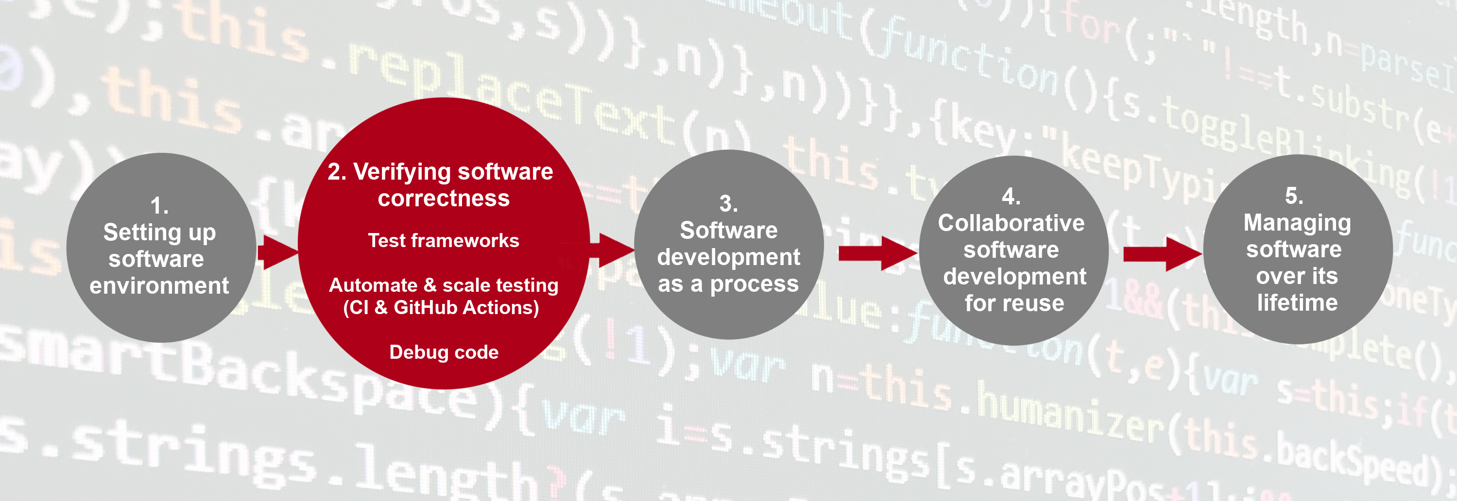
In this section we will:
- Make use of a test framework called Pytest, a free and open source Python library to help us structure and run automated tests.
- Design, write and run unit tests using Pytest to verify the correct behaviour of code and identify faults, making use of test parameterisation to increase the number of different test cases we can run.
- Automatically run a set of unit tests using GitHub Actions - a Continuous Integration infrastructure that allows us to automate tasks when things happen to our code, such as running those tests when a new commit is made to a code repository.
- Use Jupyter Lab’s integrated debugger to help us locate a fault in our code while it is running, and then fix it.
Key Points
Using testing requires us to change our practice of code development, but saves time in the long run by allowing us to more comprehensively and rapidly find faults in code, as well as giving us greater confidence in the correctness of our code.
The use of test techniques and infrastructures such as parameterisation and Continuous Integration can help scale and further automate our testing process.
Automatically Testing Software
Overview
Teaching: 30 min
Exercises: 20 minQuestions
Does the code we develop work the way it should do?
Can we (and others) verify these assertions for themselves?
To what extent are we confident of the accuracy of results that appear in publications?
Objectives
Explain the reasons why testing is important
Describe the three main types of tests and what each are used for
Implement and run unit tests to verify the correct behaviour of program functions
Introduction
Being able to demonstrate that a process generates the right results is important in any field of research, whether it’s software generating those results or not. So when writing software we need to ask ourselves some key questions:
- Does the code we develop work the way it should do?
- Can we (and others) verify these assertions for themselves?
- Perhaps most importantly, to what extent are we confident of the accuracy of results that software produces?
If we are unable to demonstrate that our software fulfills these criteria, why would anyone use it? Having well-defined tests for our software is useful for this, but manually testing software can prove an expensive process.
Automation can help, and automation where possible is a good thing - it enables us to define a potentially complex process in a repeatable way that is far less prone to error than manual approaches. Once defined, automation can also save us a lot of effort, particularly in the long run. In this episode we’ll look into techniques of automated testing to improve the predictability of a software change, make development more productive, and help us produce code that works as expected and produces desired results.
What Is Software Testing?
For the sake of argument, if each line we write has a 99% chance of being right, then a 70-line program will be wrong more than half the time. We need to do better than that, which means we need to test our software to catch these mistakes.
We can and should extensively test our software manually, and manual testing is well-suited to testing aspects such as graphical user interfaces and reconciling visual outputs against inputs. However, even with a good test plan, manual testing is very time consuming and prone to error. Another style of testing is automated testing, where we write code that tests the functions of our software. Since computers are very good and efficient at automating repetitive tasks, we should take advantage of this wherever possible.
There are three main types of automated tests:
- Unit tests are tests for fairly small and specific units of functionality, e.g. determining that a particular function returns output as expected given specific inputs.
- Functional or integration tests work at a higher level, and test functional paths through your code, e.g. given some specific inputs, a set of interconnected functions across a number of modules (or the entire code) produce the expected result. These are particularly useful for exposing faults in how functional units interact.
- Regression tests make sure that your program’s output hasn’t changed, for example after making changes your code to add new functionality or fix a bug.
For the purposes of this course, we’ll focus on unit tests. But the principles and practices we’ll talk about can be built on and applied to the other types of tests too.
Set Up a New Feature Branch for Writing Tests
We’re going to look at how to run some existing tests and also write some new ones,
so let’s ensure we’re initially on our develop branch we created earlier.
And then, we’ll create a new feature branch called test-suite off the develop branch -
a common term we use to refer to sets of tests - that we’ll use for our test writing work:
$ git checkout develop
$ git branch test-suite
$ git checkout test-suite
Good practice is to write our tests around the same time we write our code on a feature branch. But since the code already exists, we’re creating a feature branch for just these extra tests. Git branches are designed to be lightweight, and where necessary, transient, and use of branches for even small bits of work is encouraged.
Later on, once we’ve finished writing these tests and are convinced they work properly,
we’ll merge our test-suite branch back into develop.
Don’t forget to activate our venv environment, launch Jupyter Notebook and let’s see
how we can test our software for light curve analysis.
Lightcurve Data Analysis
Let’s go back to our lightcurve analysis software project.
Recall that it contains a data directory, where we have observations of presumably variable stars, namely RR Lyrae candidates, coming
from two sources: the Kepler Space Telescope and LSST Data Preview 0.
Don’t forget about the best practices
Following the best practices from the corresponding section, let’s start with creating a new notebook and drafting its structure. Using headers in the markdown cells, determine the sections of your notebook.
Solution
We can start with the following sections:
- Imports
- Params
- Data loading
- Data inspection
- Selecting light curves for a single object
- Trying the model.py functions
- Test development
If we need something else, we can always add it later.
Now let’s open our data and have a look at it. For this we will use pandas package.
Import it, open the lsst_RRLyr.pkl catalogue and have a look at the format of this table.
Don’t forget to put your code in the sections where it belongs!
import pandas as pd
lc_datasets = {}
lc_datasets['lsst'] = pd.read_pickle('data/lsst_RRLyr.pkl')
lc_datasets['lsst'].info()
lc_datasets['lsst'].head()
We can see that the dataset contains 11177 rows (‘entries’) and 12 columns.
the lc_datasets['lsst'].info() function also informs us about the types of the data in the columns,
as well as about the number of non-null values in each column.
Having a look at the top 5 rows (lc_datasets['lsst'].head()) gives us an impression of what kind
of values we have in each column.
For now there are four columns that we’ll need:
- ‘objectId’ that contains identificators of the observed objects;
- ‘band’ that informs us about the band in which the observation is made;
- ‘expMidptMJD’ that contains the time stamp of the observation;
- ‘psfMag’ that containes measured magnitudes.
Let’s assume that we want to know the maximum measured magnitudes of
the light curves in each band for a single
object. Our dataset contains observations in all bands for a number of sources, so we have
to a) pick only one source, and b) separate the observations in different bands from each other.
There are many ways of how to do this, but for the purposes of this episode we
will store the single-source observational data for each band in a dictionary
and then apply the max_mag function defined in our models.py file.
First, pick an id of the object that we will investigate.
### Pick an object
obj_id = lc_datasets['lsst']['objectId'].unique()[4]
And then store its observations in each band as items of a dictionary
lc.
### Get all the observations for this obj_id for each band
# Create an empty dict
lc = {}
# Define the bands names
bands = 'ugrizy'
# For each band create a bool array that indicates
# that this observation belongs to a certain object and is made in a
# certain band
for b in bands:
    filt_band_obj = (lc_datasets['lsst']['objectId'] == obj_id) & (
        lc_datasets['lsst']['band'] == b
    )
    # Select the observations and store in the dict 'lc'
    lc[b] = lc_datasets['lsst'][filt_band_obj]
Don’t forget about the best practices
Do you see any variables defined in the code above that you should move in some other section?
Solution
It seems very likely that we will need the variable
bandsmany times in the future. Let’s move it to the ‘Parameters’ section of the notebook.
Have a look at the resulting dictionary: you will find that each element has a key corresponding to the band name, and it’s value will contain a Pandas DataFrame with observations in this band.
Now we need to import the functions from the models.py file.
We should do it in the ‘Imports’ section.
import lcanalyzer.models as models
Pick a function from this module, for example, max_mag, and apply it to one of the light
curves.
models.max_mag(lc['g'],'psfMag')
19.183367224358136
Don’t forget about the best practices
Do you see anything in the code we just typed that can be put in the ‘Parameters’?
Solution
It is better to put the magnitude column name, ‘psfMag’, in a variable (let’s call it
colname_mag) and declare it in the ‘Parameters’ section. Why? Because chances are, in the future we will want to apply our code to another dataset with different column names, and if we continue using ‘psfMag’ across the notebook, later on we’ll have to replace it either manually, or using ‘Search’ functionality. In a large notebook both actions are likely to produce errors.
How would you check if our max_mag function works correctly?
The answer that just came to your head, in all likelyhood, sounds similar to this: “I would pass a simple DataFrame to this function and check manually that the returned maximum value is correct”. It makes perfect sense, and, perhaps, may work with a function as simple as ours:
test_input = pd.DataFrame(data=[[1, 5, 3], [7, 8, 9], [3, 4, 1]], columns=list("abc"))
test_output = 7
models.max_mag(test_input, "a") == test_output
True
But now let’s make the task more realistic and recall our original objective: to get maximum values of the light curves in all bands. We can write a function for this as well:
### Get maximum values for all bands
def calc_stat(lc, bands, mag_col):
    # Define an empty dictionary where we will store the results
    stat = {}
    # For each band get the maximum value and store it in the dictionary
    for b in bands:
        stat[b + "_max"] = models.max_mag(lc[b], mag_col)
    return stat
And then construct the test data:
df1 = pd.DataFrame(data=[[1, 5, 3], [7, 8, 9], [3, 4, 1]], columns=list("abc"))
df2 = pd.DataFrame(data=[[7, 3, 2], [8, 4, 2], [5, 6, 4]], columns=list("abc"))
df3 = pd.DataFrame(data=[[2, 6, 3], [1, 3, 6], [8, 9, 1]], columns=list("abc"))
test_input = {"df1": df1, "df2": df2, "df3": df3}
test_output = {"df1_max": 8, "df12_max": 6, "df3_max": 8}
test_output == calc_stat(test_input, ["df1", "df2", "df3"], "b")
See what kind of output this code produces.
What went wrong?
If you just copied the code above, you got
False. Try to find out what is wrong with ourcalc_statfunction.Solution
Our
calc_statfunction is fine. Ourtest_outputcontains two errors. This example highlights an important point: as well as making sure our code is returning correct answers, we also need to ensure the tests themselves are also correct. Otherwise, we may go on to fix our code only to return an incorrect result that appears to be correct. So a good rule is to make tests simple enough to understand so we can reason about both the correctness of our tests as well as our code. Otherwise, our tests hold little value.
Our crude test failed and didn’t even inform us about the reasons they failed. Surely there must be a better way to do this.
Testing Frameworks
The example above shows that manually constructing even a simple test for a fairly simple function can be tedious, and may produce new errors instead of fixing the old ones. Besides, we would like to test many functions in various scenarios, and for a complex function or a library, a test suite - a set of tests - can include dozens of tests. Obviously, running them one by one in a notebook is not a good idea, so we need a tool to automatize this process and to obtain a comprehensive report on which of the tests were passed and which failed. We’d also prefer to have something that tells us what exactly went wrong.
A solution for these tasks is called unit testing frameworks. In such a framework we define the tests we want to run as functions, and the framework automatically runs each of these functions in turn, summarising the outputs. Since most people don’t enjoy writing tests, the unit testing fraimworks aim to make it simple to:
- Add or change tests,
- Understand the tests that have already been written,
- Run those tests, and
- Understand those tests’ results.
Test results must also be reliable. If a testing tool says that code is working when it’s not, or reports problems when there actually aren’t any, people will lose faith in it and stop using it.
We will use a testing framework called pytest. It is a Python
package that can be installed, as usual, using pip:
$ python -m pip install pytest
Why Use pytest over unittest?
We could alternatively use another Python unit test framework, unittest, which has the advantage of being installed by default as part of Python. This is certainly a solid and established option, however pytest has many distinct advantages, particularly for learning, including:
- unittest requires additional knowledge of object-oriented frameworks (covered later in the course) to write unit tests, whereas in pytest these are written in simpler functions so is easier to learn
- Being written using simpler functions, pytest’s scripts are more concise and contain less boilerplate, and thus are easier to read
- pytest output, particularly in regard to test failure output, is generally considered more helpful and readable
- pytest has a vast ecosystem of plugins available if ever you need additional testing functionality
- unittest-style unit tests can be run from pytest out of the box!
A common challenge, particularly at the intermediate level, is the selection of a suitable tool from many alternatives for a given task. Once you’ve become accustomed to object-oriented programming you may find unittest a better fit for a particular project or team, so you may want to revisit it at a later date!
pytest requires that we put our tests into a separate .py file.
We already have some tests in tests/test_models.py:
"""Tests for statistics functions within the Model layer."""
import pandas as pd

def test_max_mag_integers():
    # Test that max_mag function works for integers
    from lcanalyzer.models import max_mag

    test_input_df = pd.DataFrame(data=[[1, 5, 3], [7, 8, 9], [3, 4, 1]], columns=list("abc"))
    test_input_colname = "a"
    test_output = 7

    assert max_mag(test_input_df, test_input_colname) == test_output
...
The first function represent the same test case as the one we tried first in our notebook. However, it has a different format:
- we import the function we test right inside the test function, for clarity of testing environment;
- then we specify our test input and output;
- and then we run our testing using assert keyword.
We haven’t met with assert keyword before, however, it is essential for developing,
debugging and testing of robust and reliable code. assert keyword is responsible
for checking if some condition
is true. If it is true, nothing happens and the execution of the code continues. However,
if the condition is not fullfilled, an AssertionError occurs. When you write
your own assert checks, you can use the following syntax:
assert condition, message
And testing frameworks already have their own implementations of various assertions,
for example those that can check if two dictionaries are the same (and then inform us
where exactly they differ), if two variables are of the same type and so on. Apart from that,
some other packages, including numpy and pandas, have testing modules that allow you
to compare numpy arrays, DataFrames, Series and so on.
Running Tests
Now we can run these tests in the command line using pytest:
$ python -m pytest tests/test_models.py
Here, we use -m to invoke the pytest installed module,
and specify the tests/test_models.py file to run the tests in that file explicitly.
Why Run Pytest Using
python -mand Notpytest?Another way to run
pytestis via its own command, so we could try to usepytest tests/test_models.pyon the command line instead, but this would lead to aModuleNotFoundError: No module named 'lcanalyzer'. This is because using thepython -m pytestmethod adds the current directory to its list of directories to search for modules, whilst usingpytestdoes not - thelcanalyzersubdirectory’s contents are not ‘seen’, hence theModuleNotFoundError. There are ways to get around this with various methods, but we’ve usedpython -mfor simplicity.
============================= test session starts ==============================
platform linux -- Python 3.11.5, pytest-8.0.0, pluggy-1.4.0
rootdir: /home/alex/InterPython_Workshop_Example
plugins: anyio-4.2.0
collected 2 items

tests/test_models.py ..                                                  [100%]

============================== 2 passed in 0.44s ===============================
Pytest looks for functions whose names also start with the letters ‘test_’ and runs each one.
Notice the .. after our test script:
- If the function completes without an assertion being triggered,
we count the test as a success (indicated as
.). - If an assertion fails, or we encounter an error,
we count the test as a failure (indicated as
F). The error is included in the output so we can see what went wrong.
So if we have many tests, we essentially get a report indicating which tests succeeded or failed.
Exercise: Write Some Unit Tests
We already have a couple of test cases in
tests/test_models.pythat test themax_mag()function. Looking atlcanalyzer/models.py, write at least two new test cases that test themean_mag()andmin_mag()functions, adding them totests/test_models.py. Here are some hints:
- You could choose to format your functions very similarly to
max_mag(), defining test input and expected result arrays followed by the equality assertion.- Try to choose cases that are suitably different, and remember that these functions take a DataFrame and return a float corresponding to a chosen column
- Experiment with the functions in a notebook cell in
test-development.ipynbto make sure your test result is what you expect the function to return for a given input. Don’t forget to put your new test intests/test_models.pyonce you think it’s ready!Once added, run all the tests again with
python -m pytest tests/test_models.py, and you should also see your new tests pass.Solution
def test_min_mag_negatives():
   # Test that min_mag function works for negatives
   from lcanalyzer.models import min_mag

   test_input_df = pd.DataFrame(data=[[-7, -7, -3], [-4, -3, -1], [-1, -5, -3]], columns=list("abc"))
   test_input_colname = "b"
   test_output = -7

   assert min_mag(test_input_df, test_input_colname) == test_output
def test_mean_mag_integers(): # Test that mean_mag function works for negatives from lcanalyzer.models import mean_mag test_input_df = pd.DataFrame(data=[[-7, -7, -3], [-4, -3, -1], [-1, -5, -3]], columns=list("abc")) test_input_colname = "a" test_output = -4. assert mean_mag(test_input_df, test_input_colname) == test_output
Optional Exercise: Write a Unit Test for the
calc_statfunctionIf you have some time left, extract our
calc_statfunction into themodels.pyfile and write a test for this function, using the (correct) test input and output from our experiments earlier.
The big advantage is that as our code develops we can update our test cases and commit them back, ensuring that ourselves (and others) always have a set of tests to verify our code at each step of development. This way, when we implement a new feature, we can check a) that the feature works using a test we write for it, and b) that the development of the new feature doesn’t break any existing functionality.
What About Testing for Errors?
There are some cases where seeing an error is actually the correct behaviour,
and Python allows us to test for exceptions.
Add this test in tests/test_models.py:
import pytest
def test_max_mag_strings():
    # Test for TypeError when passing a string
    from lcanalyzer.models import max_mag

    test_input_colname = "b"
    with pytest.raises(TypeError):
        error_expected = max_mag('string', test_input_colname)
Note that you need to import the pytest library at the top of our test_models.py file
with import pytest so that we can use pytest’s raises() function.
Run all your tests as before.
Since we’ve installed pytest to our environment,
we should also regenerate our requirements.txt:
$ pip3 freeze > requirements.txt
Finally, let’s commit our new test_models.py file,
requirements.txt file,
and test cases to our test-suite branch,
and push this new branch and all its commits to GitHub:
$ git add requirements.txt tests/test_models.py
$ git commit -m "Add initial test cases for mean_mag() and min_mag()"
$ git push -u origin test-suite
Why Should We Test Invalid Input Data?
Testing the behaviour of inputs, both valid and invalid, is a really good idea and is known as data validation. Even if you are developing command line software that cannot be exploited by malicious data entry, testing behaviour against invalid inputs prevents generation of erroneous results that could lead to serious misinterpretation (as well as saving time and compute cycles which may be expensive for longer-running applications). It is generally best not to assume your user’s inputs will always be rational.
What About Unit Testing in Other Languages?
Other unit testing frameworks exist for Python, including Nose2 and Unittest, and the approach to unit testing can be translated to other languages as well, e.g. pFUnit for Fortran, JUnit for Java (the original unit testing framework), Catch or gtest for C++, etc.
Key Points
The three main types of automated tests are unit tests, functional tests and regression tests.
We can write unit tests to verify that functions generate expected output given a set of specific inputs.
It should be easy to add or change tests, understand and run them, and understand their results.
We can use a unit testing framework like Pytest to structure and simplify the writing of tests in Python.
We should test for expected errors in our code.
Testing program behaviour against both valid and invalid inputs is important and is known as data validation.
Scaling Up Unit Testing
Overview
Teaching: 10 min
Exercises: 5 minQuestions
How can we make it easier to write lots of tests?
How can we know how much of our code is being tested?
Objectives
Use parameterisation to automatically run tests over a set of inputs
Use code coverage to understand how much of our code is being tested using unit tests
Introduction
We’re starting to build up a number of tests that test the same function, but just with different parameters. However, continuing to write a new function for every single test case isn’t likely to scale well as our development progresses. How can we make our job of writing tests more efficient? And importantly, as the number of tests increases, how can we determine how much of our code base is actually being tested?
Parameterising Our Unit Tests
So far, we’ve been writing a single function for every new test we need. But when we simply want to use the same test code but with different data for another test, it would be great to be able to specify multiple sets of data to use with the same test code. Test parameterisation gives us this.
So instead of writing a separate function for each different test,
we can parameterise the tests with multiple test inputs.
For example, in tests/test_models.py let us rewrite
the test_max_mag_zeros() and test_max_mag_integers()
into a single test function:
@pytest.mark.parametrize(
    "test_df, test_colname, expected",
    [
        (pd.DataFrame(data=[[1, 5, 3],
                            [7, 8, 9],
                            [3, 4, 1]],
                      columns=list("abc")),
        "a",
        7),
        (pd.DataFrame(data=[[0, 0, 0],
                            [0, 0, 0],
                            [0, 0, 0]],
                      columns=list("abc")),
        "b",
        0),
    ])
def test_max_mag(test_df, test_colname, expected):
    """Test max function works for array of zeroes and positive integers."""
    from lcanalyzer.models import max_mag
    assert max_mag(test_df, test_colname) == expected
Here, we use Pytest’s mark capability to add metadata to this specific test -
in this case, marking that it’s a parameterised test.
parameterize() function is actually a
Python decorator.
A decorator, when applied to a function,
adds some functionality to it when it is called, and here,
what we want to do is specify multiple input and expected output test cases
so the function is called over each of these inputs automatically when this test is called.
We specify these as arguments to the parameterize() decorator,
firstly indicating the names of these arguments that will be
passed to the function (test_df, test_colname, expected),
and secondly the actual arguments themselves that correspond to each of these names -
the input data (the test_df and test_colname arguments),
and the expected result (the expected argument).
In this case, we are passing in two tests to test_max_mag() which will be run sequentially.
So our first test will run max_mag() on pd.DataFrame(data=[[1, 5, 3],
[7, 8, 9],
[3, 4, 1]],
columns=list("abc")) (our test_df argument),
and check to see if it equals 7 (our expected argument) with test_colname set to 'a'.
Similarly, our second test will run max_mag()
with pd.DataFrame(data=[[0, 0, 0],
[0, 0, 0],
[0, 0, 0]],
columns=list("abc")) and check it produces 0 with test_colname set to 'b'.
The big plus here is that we don’t need to write separate functions for each of the tests - our test code can remain compact and readable as we write more tests and adding more tests scales better as our code becomes more complex.
Exercise: Write Parameterised Unit Tests
Rewrite your test functions for
mean_mag()to be parameterised, adding in new test cases. A suggestion: instead of filling the DataFrames manually, you can usenumpy.random.randint()andnumpy.random.rand()functions. When developing these tests you are likely to see a situation when the expected value is a float. In some cases your code may produce the output that has some uncertainty; how do you test such functions? For this situation,pytesthas a special function calledapprox. It allow you to assert similar values with some degree of precision; e.g.assert func(input) == pytest.approx(expected,0.01))returnsTruein when(expected-0.01)<=func(input)<=(expected+0.01). Similar solutions exist fornumpy.testingand other testing tools.Solution
...
# Parametrization for mean_mag function testing
@pytest.mark.parametrize(
    "test_df, test_colname, expected",
    [
        (pd.DataFrame(data=[[1, 5, 3],
                            [7, 8, 9],
                            [3, 4, 1]],
                      columns=list("abc")),
        "a",
        pytest.approx(3.66,0.01)),
        (pd.DataFrame(data=[[0, 0, 0],
                            [0, 0, 0],
                            [0, 0, 0]],
                      columns=list("abc")),
        "b",
        0),
    ])
def test_mean_mag(test_df, test_colname, expected):
    """Test mean function works for array of zeroes and positive integers."""
    from lcanalyzer.models import mean_mag
    assert mean_mag(test_df, test_colname) == expected
Let’s commit our revised test_models.py file and test cases to our test-suite branch
(but don’t push them to the remote repository just yet!):
$ git add tests/test_models.py
$ git commit -m "Add parameterisation mean, min, max test cases"
Code Coverage - How Much of Our Code is Tested?
Pytest can’t think of test cases for us.
We still have to decide what to test and how many tests to run.
Our best guide here is economics:
we want the tests that are most likely to give us useful information that we don’t already have.
For example, if testing our max_mag function with a DataFrame filled with integers works,
there’s probably not much point testing the same function with a DataFrame filled with other integers,
since it’s hard to think of a bug that would show up in one case but not in the other. Note, however,
that for other function this statement may be incorrect (e.g. if your function is supposed to discard values
above a certain threshold, and your test case input does not contain such values at all).
Now, we should try to choose tests that are as different from each other as possible, so that we force the code we’re testing to execute in all the different ways it can - to ensure our tests have a high degree of code coverage.
A simple way to check the code coverage for a set of tests is
to use pytest to tell us how many statements in our code are being tested.
By installing a Python package to our virtual environment called pytest-cov
that is used by Pytest and using that, we can find this out:
$ pip3 install pytest-cov
$ python -m pytest --cov=lcanalyzer.models tests/test_models.py
So here, we specify the additional named argument --cov to pytest
specifying the code to analyse for test coverage.
==================================== test session starts ====================================
platform linux -- Python 3.11.5, pytest-8.0.0, pluggy-1.4.0
rootdir: /home/alex/InterPython_Workshop_Example
plugins: anyio-4.2.0, cov-4.1.0
collected 9 items

tests/test_models_full.py .........                                                   [100%]

---------- coverage: platform linux, python 3.11.5-final-0 -----------
Name                   Stmts   Miss  Cover
------------------------------------------
lcanalyzer/models.py      12      1    92%
------------------------------------------
TOTAL                     12      1    92%


===================================== 9 passed in 0.70s =====================================
Here we can see that our tests are doing well - 92% of statements in lcanalyzer/models.py have been executed.
But which statements are not being tested?
The additional argument --cov-report term-missing can tell us:
$ python -m pytest --cov=lcanalyzer.models --cov-report term-missing tests/test_models.py
...
==================================== test session starts ====================================
platform linux -- Python 3.11.5, pytest-8.0.0, pluggy-1.4.0
rootdir: /home/alex/InterPython_Workshop_Example
plugins: anyio-4.2.0, cov-4.1.0
collected 11 items

tests/test_models.py ..                                                               [ 18%]
tests/test_models_full.py .........                                                   [100%]

---------- coverage: platform linux, python 3.11.5-final-0 -----------
Name                   Stmts   Miss  Cover   Missing
----------------------------------------------------
lcanalyzer/models.py      12      1    92%   20
----------------------------------------------------
TOTAL                     12      1    92%


==================================== 11 passed in 0.71s =====================================

...
So there’s still one statement not being tested at line 20,
and it turns out it’s in the function load_dataset().
Here we should consider whether or not to write a test for this function,
and, in general, any other functions that may not be tested.
Of course, if there are hundreds or thousands of lines that are not covered
it may not be feasible to write tests for them all.
But we should prioritise the ones for which we write tests, considering
how often they’re used,
how complex they are,
and importantly, the extent to which they affect our program’s results.
Again, we should also update our requirements.txt file with our latest package environment,
which now also includes pytest-cov, and commit it:
$ pip3 freeze > requirements.txt
$ cat requirements.txt
You’ll notice pytest-cov and coverage have been added.
Let’s commit this file and push our new branch to GitHub:
$ git add requirements.txt
$ git commit -m "Add coverage support"
$ git push origin test-suite
What about Testing Against Indeterminate Output?
What if your implementation depends on a degree of random behaviour? This can be desired within a number of applications, particularly in simulations (for example, molecular simulations) or other stochastic behavioural models of complex systems. So how can you test against such systems if the outputs are different when given the same inputs?
One way is to remove the randomness during testing. For those portions of your code that use a language feature or library to generate a random number, you can instead produce a known sequence of numbers instead when testing, to make the results deterministic and hence easier to test against. You could encapsulate this different behaviour in separate functions, methods, or classes and call the appropriate one depending on whether you are testing or not. This is essentially a type of mocking, where you are creating a “mock” version that mimics some behaviour for the purposes of testing.
Another way is to control the randomness during testing to provide results that are deterministic - the same each time. Implementations of randomness in computing languages, including Python, are actually never truly random - they are pseudorandom: the sequence of ‘random’ numbers are typically generated using a mathematical algorithm. A seed value is used to initialise an implementation’s random number generator, and from that point, the sequence of numbers is actually deterministic. Many implementations just use the system time as the default seed, but you can set your own. By doing so, the generated sequence of numbers is the same, e.g. using Python’s
randomlibrary to randomly select a sample of ten numbers from a sequence between 0-99:import random random.seed(1) print(random.sample(range(0, 100), 10)) random.seed(1) print(random.sample(range(0, 100), 10))Will produce:
[17, 72, 97, 8, 32, 15, 63, 57, 60, 83]
[17, 72, 97, 8, 32, 15, 63, 57, 60, 83]
So since your program’s randomness is essentially eliminated, your tests can be written to test against the known output. The trick of course, is to ensure that the output being testing against is definitively correct!
The other thing you can do while keeping the random behaviour, is to test the output data against expected constraints of that output. For example, if you know that all data should be within particular ranges, or within a particular statistical distribution type (e.g. normal distribution over time), you can test against that, conducting multiple test runs that take advantage of the randomness to fill the known “space” of expected results. Note that this isn’t as precise or complete, and bear in mind this could mean you need to run a lot of tests which may take considerable time.
Test Driven Development
In the previous episode we learnt how to create unit tests to make sure our code is behaving as we intended. Test Driven Development (TDD) is an extension of this. If we can define a set of tests for everything our code needs to do, then why not treat those tests as the specification.
When doing Test Driven Development, we write our tests first and only write enough code to make the tests pass. We tend to do this at the level of individual features - define the feature, write the tests, write the code. The main advantages are:
- It forces us to think about how our code will be used before we write it
- It prevents us from doing work that we don’t need to do, e.g. “I might need this later…”
- It forces us to test that the tests fail before we’ve implemented the code, meaning we don’t inadvertently forget to add the correct asserts.
You may also see this process called Red, Green, Refactor: ‘Red’ for the failing tests, ‘Green’ for the code that makes them pass, then ‘Refactor’ (tidy up) the result.
For the challenges from here on, try to first convert the specification into a unit test, then try writing the code to pass the test.
Limits to Testing
Like any other piece of experimental apparatus, a complex program requires a much higher investment in testing than a simple one. Putting it another way, a small script that is only going to be used once, to produce one figure, probably doesn’t need separate testing: its output is either correct or not. A linear algebra library that will be used by thousands of people in twice that number of applications over the course of a decade, on the other hand, definitely does. The key is identify and prioritise against what will most affect the code’s ability to generate accurate results.
It’s also important to remember that unit testing cannot catch every bug in an application, no matter how many tests you write. To mitigate this manual testing is also important. Also remember to test using as much input data as you can, since very often code is developed and tested against the same small sets of data. Increasing the amount of data you test against - from numerous sources - gives you greater confidence that the results are correct.
Our software will inevitably increase in complexity as it develops. Using automated testing where appropriate can save us considerable time, especially in the long term, and allows others to verify against correct behaviour.
Key Points
We can assign multiple inputs to tests using parametrisation.
It’s important to understand the coverage of our tests across our code.
Writing unit tests takes time, so apply them where it makes the most sense.
Github Issues and Collaborative Development
Overview
Teaching: 15 min
Exercises: 30 minQuestions
How can we keep track of identified issues and the list of tasks the team has to do?
How can we communicate within a team on code-related issues and share responsibilities?
How can we plan, prioritise and manage tasks for future development?
Objectives
Register and track progress on issues with the code in our project repository
Describe some different types of issues we can have with software
Manage communications on software development activities within the team using GitHub’s notification system Mentions
Introduction
Developing software is a project and, like most projects, it consists of multiple tasks. Keeping track of identified issues with the software, the list of tasks the team has to do, progress on each, prioritising tasks for future development, planning sprints and releases, etc., can quickly become a non-trivial task in itself. Without a good team project management process and framework, it can be hard to keep track of what’s done, or what needs doing, and particularly difficult to convey that to others in the team or share the responsibilities.
Using GitHub to Manage Issues With Software
As a piece of software is used, bugs and other issues will inevitably come to light - nothing is perfect! If you work on your code with collaborators, or have non-developer users, it can be helpful to have a single shared record of all the problems people have found with the code, not only to keep track of them for you to work on later, but to avoid people emailing you to report a bug that you already know about!
GitHub provides Issues - a framework for managing bug reports, feature requests, and lists of future work.
Go back to the home page for your InterPython_Workshop_Example repository in GitHub,
and click on the Issues tab.
You should see a page listing the open issues on your repository -
currently there should be none.

If there is no Issues tab on the page, it means they are disabled in the project settings. To fix this, go the Settings tab, then scroll down to the ‘Features’ section and select ‘Issues’ checkbox.
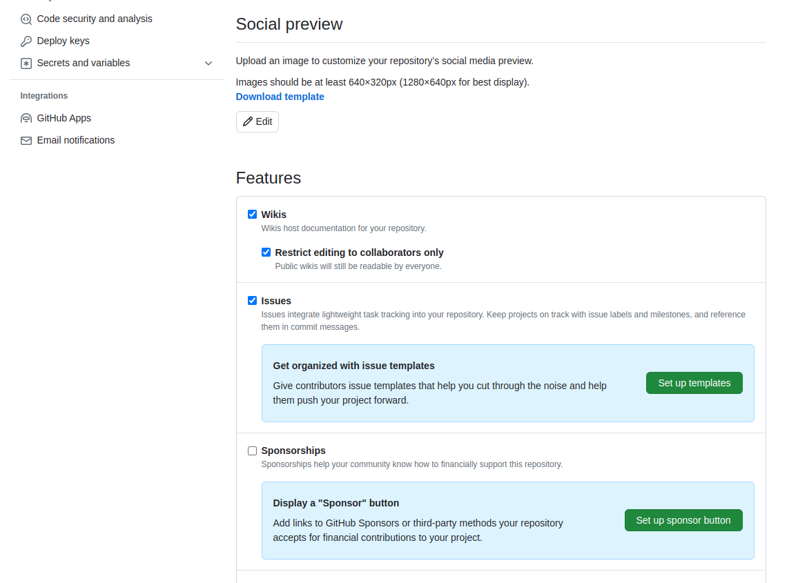
Let’s go through the process of creating a new issue.
Start by clicking the New issue button.
When you create an issue, you can add a range of details to them. They can be assigned to a specific developer for example - this can be a helpful way to know who, if anyone, is currently working to fix the issue, or a way to assign responsibility to someone to deal with it.
They can also be assigned a label. The labels available for issues can be customised, and given a colour, allowing you to see at a glance the state of your code’s issues. The default labels available in GitHub include:
bug- indicates an unexpected problem or unintended behaviordocumentation- indicates a need for improvements or additions to documentationduplicate- indicates similar or already reported issues, pull requests, or discussionsenhancement- indicates new feature requests, or if they are created by a developer, indicate planned new featuresgood first issue- indicates a good issue for first-time contributorshelp wanted- indicates that a maintainer wants help on an issue or pull requestinvalid- indicates that an issue, pull request, or discussion is no longer relevantquestion- indicates that an issue, pull request, or discussion needs more informationwontfix- indicates that work won’t continue on an issue, pull request, or discussion

You can also create your own custom labels to help with classifying issues.
There are no rules really about naming the labels -
use whatever makes sense for your project.
Some conventional custom labels include:
status:in progress (to indicate that someone started working on the issue),
status:blocked (to indicate that the progress on addressing issue is
blocked by another issue or activity), etc.
As well as highlighting problems,
the bug label can make code much more usable by
allowing users to find out if anyone has had the same problem before,
and also how to fix (or work around) it on their end.
Enabling users to solve their own problems can save you a lot of time.
In general, a good bug report should contain only one bug,
specific details of the environment in which the issue appeared
(e.g. operating system or browser, version of the software and its dependencies),
and sufficiently clear and concise steps that allow a developer to reproduce the bug themselves.
They should also be clear on what the bug reporter considers factual
(“I did this and this happened”)
and speculation
(“I think it was caused by this”).
If an error report was generated from the software itself,
it’s a very good idea to include that in the issue.
The enhancement label is a great way to communicate your future priorities
to your collaborators but also to yourself -
it’s far too easy to leave a software project for a few months to work on something else,
only to come back and forget the improvements you were going to make.
If you have other users for your code,
they can use the label to request new features,
or changes to the way the code operates.
It’s generally worth paying attention to these suggestions,
especially if you spend more time developing than running the code.
It can be very easy to end up with quirky behaviour
because of off-the-cuff choices during development.
Extra pairs of eyes can point out ways the code can be made more accessible -
the easier the code is to use, the more widely it will be adopted
and the greater impact it will have.
One interesting label is wontfix,
which indicates that an issue simply won’t be worked on for whatever reason.
Maybe the bug it reports is outside of the use case of the software,
or the feature it requests simply isn’t a priority.
This can make it clear you’ve thought about an issue and dismissed it.
Locking and Pinning Issues
The Lock conversation and Pin issue buttons are both available from individual issue pages. Locking conversations allows you to block future comments on the issue, e.g. if the conversation around the issue is not constructive or violates your team’s code of conduct. Pinning issues allows you to pin up to three issues to the top of the issues page, e.g. to emphasise their importance.
Manage Issues With Your Code Openly
Having open, publicly-visible lists of the limitations and problems with your code is incredibly helpful. Even if some issues end up languishing unfixed for years, letting users know about them can save them a huge amount of work attempting to fix what turns out to be an unfixable problem on their end. It can also help you see at a glance what state your code is in, making it easier to prioritise future work!
Exercise: Our First Issue!
Individually, with a critical eye, think of an aspect of the code you have developed so far that needs improvement. It could be a bug, for example, or an absent docstring, or an enhancement. In GitHub, enter the details of the issue and select
Submit new issue. Add a label to your issue, if appropriate.Time: 5 mins
Solution
For example, “Add arguments description to the docstring of the mean_mag function” could be a good first issue, with a label
documentation.
Issue (and Pull Request) Templates
GitHub also allows you to set up issue and pull request templates for your software project. Such templates provide a structure for the issue/pull request descriptions, and/or prompt issue reporters and collaborators to fill in answers to pre-set questions. They can help contributors raise issues or submit pull requests in a way that is clear, helpful and provides enough information for maintainers to act upon (without going back and forth to extract it). GitHub provides a range of default templates, but you can also write your own.
Using GitHub’s Notifications & Referencing System to Communicate
GitHub implements a comprehensive notifications system to keep the team up-to-date with activities in your code repository and notify you when something happens or changes in your software project. You can choose whether to watch or unwatch an individual repository, or can choose to only be notified of certain event types such as updates to issues, pull requests, direct mentions, etc. GitHub also provides an additional useful notification feature for collaborative work - Mentions. In addition to referencing team members (which will result in an appropriate notification), GitHub allows us to reference issues, pull requests and comments from one another - providing a useful way of connecting things and conversations in your project.
Referencing Team Members Using Mentions
The mention system notifies team members when somebody else references them in an issue, comment or pull request - you can use this to notify people when you want to check a detail with them, or let them know something has been fixed or changed (much easier than writing out all the same information again in an email).
You can use the mention system to link to/notify an individual GitHub account or a whole team for notifying multiple people. Typing @ in GitHub will bring up a list of all accounts and teams linked to the repository that can be “mentioned”. People will then receive notifications based on their preferred notification methods - e.g. via email or GitHub’s User Interface.
Referencing Issues, Pull Requests and Comments
GitHub also lets you mention/reference one issue or pull request from another (and people “watching” these will be notified of any such updates). Whilst writing the description of an issue, or commenting on one, if you type # you should see a list of the issues and pull requests on the repository. They are coloured green if they’re open, or white if they’re closed. Continue typing the issue number, and the list will narrow down, then you can hit Return to select the entry and link the two. For example, if you realise that several of your bugs have common roots, or that one enhancement can’t be implemented before you’ve finished another, you can use the mention system to indicate the depending issue(s). This is a simple way to add much more information to your issues.
While not strictly notifying anyone,
GitHub lets you also reference individual comments and commits.
If you click the ... button on a comment,
from the drop down list you can select to Copy link
(which is a URL that points to that comment that can be pasted elsewhere)
or to Reference [a comment] in a new issue
(which opens a new issue and references the comment by its URL).
Within a text box for comments, issue and pull request descriptions,
you can reference a commit by pasting its long, unique identifier
(or its first few digits which uniquely identify it)
and GitHub will render it nicely using the identifier’s short form
and link to the commit in question.
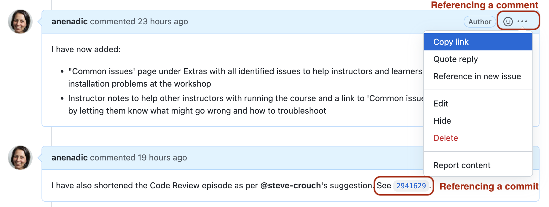
Exercise: Collaborative Traning!
Following the organizers’ instructions, go into breakout rooms. Share your GitHub accounts with each other, and spend about 10 minutes creating issues for each other’s workshop project repositories. The issues may include missing or incomplete docstrings, structure of the notebooks, lacking unit tests and so on. When appropriate, use markdown formatting for making your issues easier to understand.
After that, go to your own repository and inspect issues that your collegues created. Assign appropriate labels and comment on a few issues, mentioning your team members using the
@notation - e.g. to ask them a question or a clarification on something or to do some additional work.Pick one of the smaller issues and create a commit to fix it. Use issue or commit referencing to link them and close the issue as completed.
Time: 25 mins
You Are Also a User of Your Code
This section focuses a lot on how issues and mentions can help communicate the current state of the code to others and document what conversations were held around particular issues. As a sole developer, and possibly also the only user of the code, you might be tempted to not bother with recording issues, comments and new features as you don’t need to communicate the information to anyone else.
Unfortunately, human memory isn’t infallible! After spending six months on a different topic, it’s inevitable you’ll forget some of the plans you had and problems you faced. Not documenting these things can lead to you having to re-learn things you already put the effort into discovering before. Also, if others are brought on to the project at a later date, the software’s existing issues and potential new features are already in place to build upon.
Key Points
We should use GitHub’s Issues to keep track of software problems and other requests for change - even if we are the only developer and user.
GitHub’s Mentions play an important part in communicating between collaborators and is used as a way of alerting team members of activities and referencing one issue/pull requests/comment/commit from another.
Continuous Integration for Automated Testing
Overview
Teaching: 45 min
Exercises: 0 minQuestions
How can I automate the testing of my repository’s code in a way that scales well?
What can I do to make testing across multiple platforms easier?
Objectives
Describe the benefits of using Continuous Integration for further automation of testing
Enable GitHub Actions Continuous Integration for public open source repositories
Use continuous integration to automatically run unit tests and code coverage when changes are committed to a version control repository
Use a build matrix to specify combinations of operating systems and Python versions to run tests over
Introduction
So far we’ve been manually running our tests as we require. Once we’ve made a change, or added a new feature with accompanying tests, we can re-run our tests, giving ourselves (and others who wish to run them) increased confidence that everything is working as expected. Now we’re going to take further advantage of automation in a way that helps testing scale across a development team with very little overhead, using Continuous Integration.
What is Continuous Integration?
The automated testing we’ve done so far only takes into account the state of the repository we have on our own machines. In a software project involving multiple developers working and pushing changes on a repository, it would be great to know holistically how all these changes are affecting our codebase without everyone having to pull down all the changes and test them. If we also take into account the testing required on different target user platforms for our software and the changes being made to many repository branches, the effort required to conduct testing at this scale can quickly become intractable for a research project to sustain.
Continuous Integration (CI) aims to reduce this burden by further automation, and automation - wherever possible - helps us to reduce errors and makes predictable processes more efficient. The idea is that when a new change is committed to a repository, CI clones the repository, builds it if necessary, and runs any tests. Once complete, it presents a report to let you see what happened.
There are many CI infrastructures and services, free and paid for, and subject to change as they evolve their features. We’ll be looking at GitHub Actions - which unsurprisingly is available as part of GitHub.
Continuous Integration with GitHub Actions
A Quick Look at YAML
YAML is a text format used by GitHub Action workflow files. It is also increasingly used for configuration files and storing other types of data, so it’s worth taking a bit of time looking into this file format.
YAML (a recursive acronym which stands for “YAML Ain’t Markup Language”) is a language designed to be human readable. A few basic things you need to know about YAML to get started with GitHub Actions are key-value pairs, arrays, maps and multi-line strings.
So firstly, YAML files are essentially made up of key-value pairs,
in the form key: value, for example:
name: Kilimanjaro
height_metres: 5892
first_scaled_by: Hans Meyer
In general, you don’t need quotes for strings,
but you can use them when you want to explicitly distinguish between numbers and strings,
e.g. height_metres: "5892" would be a string,
but in the above example it is an integer.
It turns out Hans Meyer isn’t the only first ascender of Kilimanjaro,
so one way to add this person as another value to this key is by using YAML arrays,
like this:
first_scaled_by:
- Hans Meyer
- Ludwig Purtscheller
An alternative to this format for arrays is the following, which would have the same meaning:
first_scaled_by: [Hans Meyer, Ludwig Purtscheller]
If we wanted to express more information for one of these values we could use a feature known as maps (dictionaries/hashes), which allow us to define nested, hierarchical data structures, e.g.
...
height:
  value: 5892
  unit: metres
  measured:
    year: 2008
    by: Kilimanjaro 2008 Precise Height Measurement Expedition
...
So here, height itself is made up of three keys value, unit, and measured,
with the last of these being another nested key with the keys year and by.
Note the convention of using two spaces for tabs, instead of Python’s four.
We can also combine maps and arrays to describe more complex data. Let’s say we want to add more detail to our list of initial ascenders:
...
first_scaled_by:
- name: Hans Meyer
  date_of_birth: 22-03-1858
  nationality: German
- name: Ludwig Purtscheller
  date_of_birth: 22-03-1858
  nationality: Austrian
So here we have a YAML array of our two mountaineers, each with additional keys offering more information.
GitHub Actions also makes use of | symbol to indicate a multi-line string
that preserves new lines. For example:
shakespeare_couplet: |
  Good night, good night. Parting is such sweet sorrow
  That I shall say good night till it be morrow.
They key shakespeare_couplet would hold the full two line string,
preserving the new line after sorrow.
As we’ll see shortly, GitHub Actions workflows will use all of these.
Defining Our Workflow
With a GitHub repository there’s a way we can set up CI
to run our tests automatically when we commit changes.
Let’s do this now by adding a new file to our repository whilst on the test-suite branch.
First, create the new directories .github/workflows:
$ mkdir -p .github/workflows
This directory is used specifically for GitHub Actions,
allowing us to specify any number of workflows that can be run under a variety of conditions,
which is also written using YAML.
So let’s add a new YAML file called main.yml
(note it’s extension is .yml without the a)
within the new .github/workflows directory:
name: CI

# We can specify which Github events will trigger a CI build
on: push

# now define a single job 'build' (but could define more)
jobs:

  build:

    # we can also specify the OS to run tests on
    runs-on: ubuntu-latest

    # a job is a seq of steps
    steps:

    # Next we need to checkout out repository, and set up Python
    # A 'name' is just an optional label shown in the log - helpful to clarify progress - and can be anything
    - name: Checkout repository
      uses: actions/checkout@v4

    - name: Set up Python
      uses: actions/setup-python@v5
      with:
        python-version: "3.11"

    - name: Install Python dependencies
      run: |
        python -m pip install --upgrade pip
        pip install -r requirements.txt

    - name: Test with PyTest
      run: |
        python -m pytest --cov=lcanalyzer.models tests/test_models.py
Note: be sure to create this file as main.yml
within the newly created .github/workflows directory,
or it won’t work!
So as well as giving our workflow a name - CI -
we indicate with on that we want this workflow to run when we push commits to our repository.
The workflow itself is made of a single job named build,
and we could define any number of jobs after this one if we wanted,
and each one would run in parallel.
Next, we define what our build job will do.
With runs-on we first state which operating systems we want to use,
in this case just Ubuntu for now.
We’ll be looking at ways we can scale this up to testing on more systems later.
Lastly, we define the steps that our job will undertake in turn,
to set up the job’s environment and run our tests.
You can think of the job’s environment initially as a blank slate:
much like a freshly installed machine (albeit virtual) with very little installed on it,
we need to prepare it with what it needs to be able to run our tests.
Each of these steps are:
- Checkout repository for the job:
usesindicates that want to use a GitHub Action calledcheckoutthat does this - Set up Python 3.11:
here we use the
setup-pythonAction, indicating that we want Python version 3.11. Note we specify the version within quotes, to ensure that this is interpreted as a complete string. Otherwise, if we wanted to test against for example Python 3.10, by specifying3.10without the quotes, it would be interpreted as the number3.1which - although it’s the same number as3.10- would be interpreted as the wrong version! - Install latest version of pip, dependencies, and our lightcurves package:
In order to locally install our
lcanalyzerpackage it’s good practice to upgrade the version of pip that is present first, then we use pip to install our package dependencies. Once installed, we can usepip3 install -e .as before to install our own package. We userunhere to run theses commands in the CI shell environment - Test with PyTest: lastly, we run
python -m pytest, with the same arguments we used manually before
What about other Actions?
Our workflow here uses standard GitHub Actions (indicated by
actions/*). Beyond the standard set of actions, others are available via the GitHub Marketplace. It contains many third-party actions (as well as apps) that you can use with GitHub for many tasks across many programming languages, particularly for setting up environments for running tests, code analysis and other tools, setting up and using infrastructure (for things like Docker or Amazon’s AWS cloud), or even managing repository issues. You can even contribute your own.
Triggering a Build on GitHub Actions
Now if we commit and push this change a CI run will be triggered:
$ git add .github
$ git commit -m "Add GitHub Actions configuration"
$ git push
Since we are only committing the GitHub Actions configuration file
to the test-suite branch for the moment,
only the contents of this branch will be used for CI.
We can pass this file upstream into other branches (i.e. via merges) when we’re happy it works,
which will then allow the process to run automatically on these other branches.
This again highlights the usefulness of the feature-branch model -
we can work in isolation on a feature until it’s ready to be passed upstream
without disrupting development on other branches,
and in the case of CI,
we’re starting to see its scaling benefits across a larger scale development team
working across potentially many branches.
Checking Build Progress and Reports
Handily, we can see the progress of the build from our repository on GitHub
by selecting the test-suite branch from the dropdown menu
(which currently says main),
and then selecting commits
(located just above the code directory listing on the right,
alongside the last commit message and a small image of a timer).


You’ll see a list of commits for this branch,
and likely see an orange marker next to the latest commit
(clicking on it yields Some checks haven’t completed yet)
meaning the build is still in progress.
This is a useful view, as over time, it will give you a history of commits,
who did them, and whether the commit resulted in a successful build or not.
Hopefully after a while, the marker will turn into a green tick indicating a successful build.
Clicking it gives you even more information about the build,
and selecting Details link takes you to a complete log of the build and its output.
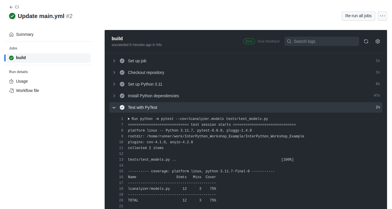
The logs are actually truncated; selecting the arrows next to the entries -
which are the name labels we specified in the main.yml file -
will expand them with more detail, including the output from the actions performed.
GitHub Actions offers these continuous integration features as a completely free service for public repositories, and supplies 2000 build minutes a month on as many private repositories that you like. Paid levels are available too.
Scaling Up Testing Using Build Matrices
Now we have our CI configured and building, we can use a feature called build matrices which really shows the value of using CI to test at scale.
Suppose the intended users of our software use either Ubuntu, Mac OS, or Windows, and either have Python version 3.10 or 3.11 installed, and we want to support all of these. Assuming we have a suitable test suite, it would take a considerable amount of time to set up testing platforms to run our tests across all these platform combinations. Fortunately, CI can do the hard work for us very easily.
Using a build matrix we can specify testing environments and parameters (such as operating system, Python version, etc.) and new jobs will be created that run our tests for each permutation of these.
Let’s see how this is done using GitHub Actions.
To support this, we define a strategy as
a matrix of operating systems and Python versions within build.
We then use matrix.os and matrix.python-version to reference these configuration possibilities
instead of using hardcoded values -
replacing the runs-on and python-version parameters
to refer to the values from the matrix.
So, our .github/workflows/main.yml should look like the following:
...
# now define a single job 'build' (but could define more)
jobs:

  build:

    strategy:
      matrix:
        os: [ubuntu-latest, macos-latest, windows-latest]
        python-version: ["3.10", "3.11"]

    runs-on: ${{ matrix.os }}

...

    # a job is a seq of steps
    steps:

    # Next we need to checkout out repository, and set up Python
    # A 'name' is just an optional label shown in the log - helpful to clarify progress - and can be anything
    - name: Checkout repository
      uses: actions/checkout@v4

    - name: Set up Python 3.11
      uses: actions/setup-python@v5
      with:
        python-version: ${{ matrix.python-version }}
...
The ${{ }} are used as a means to reference configuration values from the matrix.
This way, every possible permutation of Python versions 3.10 and 3.11 with the latest
versions of Ubuntu, Mac OS and Windows operating systems will be tested and we can expect 6 build jobs in total.
Let’s commit and push this change and see what happens:
$ git add .github/workflows/main.yml
$ git commit -m "Add GA build matrix for os and Python version"
$ git push
If we go to our GitHub build now, we can see that a new job has been created for each permutation.
Note all jobs running in parallel (up to the limit allowed by our account) which potentially saves us a lot of time waiting for testing results. Overall, this approach allows us to massively scale our automated testing across platforms we wish to test.
Merging Back to develop Branch
Now we’re happy with our test suite, we can merge this work
(which currently only exist on our test-suite branch)
with our parent develop branch.
Again, this reflects us working with impunity on a logical unit of work,
involving multiple commits,
on a separate feature branch until it’s ready to be escalated to the develop branch:
$ git checkout develop
$ git merge test-suite
Then, assuming no conflicts we can push these changes back to the remote repository as we’ve done before:
$ git push origin develop
Now these changes have migrated to our parent develop branch,
develop will also inherit the configuration to run CI builds,
so these will run automatically on this branch as well.
This highlights a big benefit of CI when you perform merges (and apply pull requests).
As new branch code is merged into upstream branches like develop and main
these newly integrated code changes are automatically tested together with existing code -
which of course may also have changed in the meantime!
Key Points
Continuous Integration can run tests automatically to verify changes as code develops in our repository.
CI builds are typically triggered by commits pushed to a repository.
We need to write a configuration file to inform a CI service what to do for a build.
We can specify a build matrix to specify multiple platforms and programming language versions to test against
Builds can be enabled and configured separately for each branch.
We can run - and get reports from - different CI infrastructure builds simultaneously.
Issue Diagnostics with a Debugger and Other Tools
Overview
Teaching: 30 min
Exercises: 20 minQuestions
Once we know our program has errors, how can we locate them in the code?
How can we make our programs more resilient to failure?
Objectives
Use a debugger to explore behaviour of a running program
Describe and identify edge and corner test cases and explain why they are important
Apply error handling and defensive programming techniques to improve robustness of a program
Integrate linting tool style checking into a continuous integration job
Introduction
Unit testing can tell us something is wrong in our code
and give a rough idea of where the error is
by which test(s) are failing.
But it does not tell us exactly where the problem is (i.e. what line of code),
or how it came about.
The process of finding out what causes errors in our code is called debugging.
There are numerous toold and methods for doing this, and in all likelyhood,
you are already using some of them. Perhaps the most common way of debugging your
Python code, especially when the project is relatively simple, is to use print
statements for inspecting intermediate values of the variables. Jupyter Lab with its
cell-by-cell workflow especially encourages this kind of debugging. Another approach
is to split a larger piece of code into smaller chunks and check them piece by piece.
However, there is more advanced tool for this, called debugger.
Setting the Scene
Let us add a new function to our jupyter notebook called calc_stats()
that will calculate for us all three statistical indicators (min, max and mean) for all
bands of our light curve.
(Make sure you create a new feature branch for this work off your develop branch.)
def calc_stats(lc, bands, mag_col):
    # Calculate max, mean and min values for all bands of a light curve
    stats = {}
    for b in bands:
        stat = {}
        stat["max"] = models.max_mag(lc[b], mag_col)
        stat["mean"] = models.max_mag(lc[b], mag_col)
        stat["min"] = models.mean_mag(lc[b], mag_col)
        stats[b] = stat
    return pd.DataFrame.from_records(stats)
Note: there are intentional mistakes in the above code, which will be detected by further testing and code style checking below so bear with us for the moment!
This code accepts a dictionary of DataFrames that contain observations of a single object in all bands.
Then this code iterates through the bands, calculating the requested statistical values and storing them
in a dictionary. At the end, these dictionaries are converted into a DataFrame, where column names are the
keys of the original lc dictionary, and the index (‘row names’) are the names of the statistics (‘max’,
‘mean’ and ‘min’). Pass one of our previously designed light curves to this function
to see that the result is an accurate and informative pandas table.
Can’t we save them directly into a DataFrame?
Technically, we can. However, editing DataFrames row by row or element by element is inefficient from the computational point of view. For this reason, when creating a frame row by row is inevitable, storing data in a list, dictionary or array and then converting them in a DataFrame is the preferred solution. It is also worth noting that in many cases iterations in a loop through the rows of some kind of a table can be avoided entirely with a better design of the algorithm.
Now let’s design a test case for this function:
test_cols = list("abc")
test_dict = {}
test_dict["df0"] = pd.DataFrame(
    data=[[8, 8, 0],
          [0, 1, 1],
          [2, 3, 1],
          [7, 9, 7]], columns=test_cols
)
test_dict["df1"] = pd.DataFrame(
    data=[[3, 8, 2],
          [3, 8, 0],
          [3, 9, 8],
          [8, 2, 5]], columns=test_cols
)
test_dict["df2"] = pd.DataFrame(
    data=[[8, 4, 3],
          [7, 6, 3],
          [4, 2, 9],
          [6, 4, 0]], columns=test_cols
)
Remember, that we don’t have to fill the data manually, but can use built-in numpy
random generator. For example, for the data above size = (4,3); np.random.randint(0, 10, size)
was used.
The expected output for these data will look like this:
test_output = pd.DataFrame(data=[[9,9,6],[5.25,6.75,4.],[1,2,2]],columns=['df0','df1','df2'],index=['max','mean','min'])
Finally, we can use assert statement to check if our function produces what we expect…
assert calc_stats(test_dict, test_dict.keys(), 'b') == test_output
…and get a ValueError:
...
ValueError: The truth value of a DataFrame is ambiguous. Use a.empty, a.bool(), a.item(), a.any() or a.all().
The reason for this is that assert takes a condition that produces a single boolean value,
but using == for two DataFrames results in an element-wise comparison and produces a DataFrame
filled with booleans.
This is the case when we need to use a more powerful assert function, the one that is developed specifically
for a certain variable type. Pandas has its own module called testing that contains a number of type-specific
assert functions. Let’s import this module:
import pandas.testing as pdt
And use assert_frame_equal function that can compare DataFrames in a meaningful way:
pdt.assert_frame_equal(calc_stats(test_dict, test_dict.keys(), 'b'),
                              test_output,
                             check_exact=False,
                             atol=0.01)
The first two arguments of this function are just what we would expect: the call of our calc_stats
function and the expected test_output. assert_frame_equal will be comparing these two DataFrames.
The next two arguments allow this function to compare the DataFrames with only some degree of precision.
This precision is determined by the argument atol, which stands for ‘absolute tolerance’. The DataFrames
will be considered equal if their elements differ no more than by atol value. This is similar to the
pytest.approx that we encountered in the previous episodes.
This assertion is falining with an error message that does not give many clues as to what went wrong.
...
AssertionError: DataFrame.iloc[:, 0] (column name="df0") are different

DataFrame.iloc[:, 0] (column name="df0") values are different (66.66667 %)
[index]: [max, mean, min]
[left]:  [9.0, 9.0, 5.25]
[right]: [9.0, 5.25, 1.0]
At positional index 1, first diff: 9.0 != 5.25
Apparently, there are differences between the two DataFrames in the column ‘df0’;
the values in the ‘max’ row are the same, but the ‘mean’ and ‘min’ values are different.
Instead of adding print statements in our function and executing it again and again, let’s
use a debugger at this point to see what is going on and why the function failed.
Debugging in Jupyter Lab
The debugger in essence is a software for inspecting the changes that happen to
the variables, memory allocation and other resources when your code is being executed.
This software can be a simple package that will print something useful in the console
(in fact, Python has such a package which is called pdb)
or a GUI tool, which is usually integrated into the IDE. To enable the debugger in Jupyter Lab,
click on a small bug pictogram in the top right corner of your notebook tab (it will turn orange,
indicating that debugging mode is active), and then open the debugger right-side panel
(also marked with a bug pictogram).
The debugger panel contains five sections:
- Variables. This is the place where all variables, user-defined or not, can be inspected in all the details. You can switch between the tree view and table view using the buttons in the top right corner of this section. The tree view provides you with more information, for example, you can see the full list of methods available for this object. However, table view is more concise and simple for understanding, as it contains only variable names, types and values.
- Callstack. Here you can trace the chain of function calls that brings you to the breakpoint - a stopping place in the code, that you define manually.
- Breakpoints. Here you will find the list of your breakpoints.
- Sources. The currently debugged code will be shown here.
- Kernel sources. Through this section you can inspect the source code of all modules that are currently available to the kernel.

Turning on the debugger and setting the breakpoint. The 'Variables' section in the table view shows all previously defined variables.
To inspect how our variables change during code execution and find the source of the error,
we should set a breakpoint somewhere before the error occurs. To be on the safe side, let’s put the
breakpoint on the line where we define our stat dictionary. Now we should go to the cell where we execute
our assertion of the function output and the expected output and run it.
The execution of the code will start, but then pause once the interpreter reaches the breakpoint.
Here we should start paying attention to the ‘Variables’ section. At this point, we have only the variables
that we passed to the function as the arguments, and an empty stats dictionary. In the ‘Callstack’
section, let’s click on the Next button (the third one in the row; alternatively you can press F10).
The interpreter will move to the next line, and we will see a new variable in the ‘Variables’ - an empty dict
called stat.
Keep clicking Next and moving through the code. You’ll notice that some elements appear in the stat dictionary:
first max with value 9, then mean with value 9…

Finding the error
Wait a second. mean equals 9? That can’t be right.
Here we found the line in which an error occurs. After looking at it closely we will notice that we used the wrong function, and if we keep going through the code with the debugger, we’ll notice that the next line contains an error as well.
Case solved! Now we can Terminate the debugging (by clicking on a ‘Stop’ button in the ‘Callstack’ section), turn off the debugger
(by clicking on the orange bug sign in the notebook tab; do not skip this step as debugging mode affects performance) and fix the errors.
Is this really easier than
When using the debugger for the first time, it may appear that it is more complicated and cumbersome than just inserting in the code
Optional Exercise: Extracting the Functions into
.pyFilesFollowing the best practices that you learned on Day 1, put the
calc_statsfunction into themodels.pyfile and convert the assertion for this function into a proper test in thetests/test_models.py.
Corner or Edge Cases
The test cases that we have written so far are parameterised with a fairly standard DataFrames filled with random integers or floats. However, when writing your test cases, it is important to consider parameterising them by unusual or extreme values, in order to test all the edge or corner cases that your code could be exposed to in practice. Generally speaking, it is at these extreme cases that you will find your code failing, so it’s beneficial to test them beforehand.
What is considered an “edge case” for a given component depends on
what that component is meant to do.
For numerical values, extreme cases could be zeros,
very large or small values,
not-a-number (NaN) or infinity values.
Since we are specifically considering arrays of values,
an edge case could be that all the numbers of the array are equal.
For all the given edge cases you might come up with, you should also consider their likelihood of occurrence. It is often too much effort to exhaustively test a given function against every possible input, so you should prioritise edge cases that are likely to occur. Let’s consider a new function, which purpose is to normalize a single light curve:
def normalize_lc(df,mag_col):
    # Normalize a single light curve
    min = min_mag(df,mag_col)
    max = max_mag((df-min),mag_col)
    lc = (df[mag_col]-min)/max
    return lc
For a function like this, a common edge case might be the occurrence of zeros, and the case where all the values of the array are the same. Indeed, if we passed to such a function a ‘light curve’ where all measurements are zeros, we would expect to have zeros in return. However, since we have division in this function, it will return and array of ‘NaN’ instead of this.
With this in mind,
let us create a test test_normalize_lc with parametrization
corresponding to an input array of random integers, an input array of all 0,
and an input array of all 1.
# Parametrization for normalize_lc function testing
@pytest.mark.parametrize(
    "test_input_df, test_input_colname, expected",
    [
        (pd.DataFrame(data=[[8, 9, 1],
                            [1, 4, 1],
                            [1, 2, 4],
                            [1, 4, 1]],
                      columns=list("abc")),
        "b",
        pd.Series(data=[1,0.285,0,0.285])),
        (pd.DataFrame(data=[[1, 1, 1],
                            [1, 1, 1],
                            [1, 1, 1],
                            [1, 1, 1]],
                      columns=list("abc")),
        "b",
        pd.Series(data=[0.,0.,0.,0.])),
        (pd.DataFrame(data=[[0, 0, 0],
                            [0, 0, 0],
                            [0, 0, 0],
                            [0, 0, 0]],
                      columns=list("abc")),
        "b",
         pd.Series(data=[0.,0.,0.,0.])),
    ])
def test_normalize_lc(test_input_df, test_input_colname, expected):
    """Test how normalize_lc function works for arrays of positive integers."""
    from lcanalyzer.models import normalize_lc
    import pandas.testing as pdt
    pdt.assert_series_equal(normalize_lc(test_input_df,test_input_colname),expected,check_exact=False,atol=0.01,check_names=False)
Pay attention, that since this our normalize_lc function returns a pandas.Series, we have to use the corresponding assert function
(pdt.assert_series_equal). Another thing to pay attention to is the arguments of this function. Not only we specify the atol for
ensuring that there will be no issues when comparing floats, but also set check_names=False, since by default the Series returned from
the normalize_lc function will have the name of the column for which we performed the normalization. Custom assert functions, such as
assert_series_equal, often take a large number of arguments that specify which parameters of the objects have to be compared. E.g. you can
opt out of comparing the dtypes of a Series, the column orders of a DataFrame and so on.
Running the tests now from the command line results in the following assertion error,
due to the division by zero as we predicted. Note that not only the test case with all zeros
fails, but also the test with all ones too, due to the extraction of the min value!
E   AssertionError: Series are different
E
E   Series values are different (100.0 %)
E   [index]: [0, 1, 2, 3]
E   [left]:  [nan, nan, nan, nan]
E   [right]: [0.0, 0.0, 0.0, 0.0]
E   At positional index 0, first diff: nan != 0.0

testing.pyx:173: AssertionError
====================================================================================== short test summary info ======================================================================================
FAILED tests/test_models_full.py::test_normalize_lc[test_input_df1-b-expected1] - AssertionError: Series are different
FAILED tests/test_models_full.py::test_normalize_lc[test_input_df2-b-expected2] - AssertionError: Series are different
How can we fix this? For example, we can replace all the NaNs in the
return Series with zeros using pandas function fillna.
...
def normalize_lc(df,mag_col):
    # Normalize a single light curve
    min = min_mag(df,mag_col)
    max = max_mag((df-min),mag_col)
    lc = (df[mag_col]-min)/max
    lc = lc.fillna(0)
    return lc
...
Defensive Programming
In the previous section, we made a few design choices for our normalize_lc function:
- We are implicitly converting any
NaNto 0, - Normalising a constant array of magnitudes in an identical array of 0s,
- We don’t warn the user of any of these situations.
This could have be handled differently. We might decide that we do not want to silently make these changes to the data, but instead to explicitly check that the input data satisfies a given set of assumptions (e.g. no negative values or no values outside of a certain range) and raise an error if this is not the case. Then we can proceed with the normalisation, confident that our normalisation function will work correctly.
Checking that input to a function is valid via a set of preconditions
is one of the simplest forms of defensive programming
which is used as a way of avoiding potential errors.
Preconditions are checked at the beginning of the function
to make sure that all assumptions are satisfied.
These assumptions are often based on the value of the arguments, like we have already discussed.
However, in a dynamic language like Python
one of the more common preconditions is to check that the arguments of a function
are of the correct type.
Currently there is nothing stopping someone from calling normalize_lc with
a string, a dictionary, or another object that is not a DataFrame, or from
passing a DataFrame filled with strings or lists.
As an example, let us change the behaviour of the normalize_lc() function
to raise an error if some magnitudes are smaller than ‘-90’ (since in astronomical data ‘-99.’ or ‘-99.9’ are
common filler values for ‘NaNs’).
Edit our function by adding a precondition check like so:
...
    if any(df[mag_col].abs() > 90):
        raise ValueError(mag_col+' contains values with abs() larger than 90!')
...
We can then modify our test function
to check that the function raises the correct exception - a ValueError -
when input to the test contains ‘-99.9’ values.
The ValueError exception
is part of the standard Python library
and is used to indicate that the function received an argument of the right type,
but of an inappropriate value.
In lcanalyzer/models.py
def normalize_lc(df,mag_col):
    # Normalize a light curve
    if any(df[mag_col].abs() > 90):
        raise ValueError(mag_col+' contains values with abs() larger than 90!')
    min = min_mag(df,mag_col)
    max = max_mag((df-min),mag_col)
    lc = (df[mag_col]-min)/max
    lc = lc.fillna(0)
    return lc
Here we added a condition that if our input data contains values that are larger than 90 or smaller than -90,
we should raise a ValueError with the corresponding message.
In tests/test_models.py
# Parametrization for normalize_lc function testing with ValueError
@pytest.mark.parametrize(
    "test_input_df, test_input_colname, expected, expected_raises",
    [
        (pd.DataFrame(data=[[8, 9, 1],
                            [1, 4, 1],
                            [1, 2, 4],
                            [1, 4, 1]],
                      columns=list("abc")),
        "b",
        pd.Series(data=[1,0.285,0,0.285]),
        None),
        (pd.DataFrame(data=[[1, 1, 1],
                            [1, 1, 1],
                            [1, 1, 1],
                            [1, 1, 1]],
                      columns=list("abc")),
        "b",
        pd.Series(data=[0.,0.,0.,0.]),
        None),
        (pd.DataFrame(data=[[0, 0, 0],
                            [0, 0, 0],
                            [0, 0, 0],
                            [0, 0, 0]],
                      columns=list("abc")),
        "b",
        pd.Series(data=[0.,0.,0.,0.]),
        None),
        (pd.DataFrame(data=[[8, 9, 1],
                            [1, -99.9, 1],
                            [1, 2, 4],
                            [1, 4, 1]],
                      columns=list("abc")),
        "b",
        pd.Series(data=[1,0.285,0,0.285]),
        ValueError),
    ])
def test_normalize_lc(test_input_df, test_input_colname, expected,expected_raises):
    """Test how normalize_lc function works for arrays of positive integers."""
    from lcanalyzer.models import normalize_lc
    import pandas.testing as pdt
    if expected_raises is not None:
        with pytest.raises(expected_raises):
            pdt.assert_series_equal(normalize_lc(test_input_df,test_input_colname),expected,check_exact=False,atol=0.01,check_names=False)
    else:
        pdt.assert_series_equal(normalize_lc(test_input_df,test_input_colname),expected,check_exact=False,atol=0.01,check_names=False)
And in the test_models we had to add to our parametrization a new function argument
called expected_raises, which is equal to None
for the test cases where our function should not invoke any raises. In the testing function itself
we are adding an if statement to separately handling the situation when a raise is expected.
Be sure to commit your changes so far and push them to GitHub.
Optional Exercise: Add a Precondition to Check the Correct Type and Column Names
Add preconditions to check that input data is
DataFrameobject and that its columns contain the column for which we have to perform normalization. Add corresponding tests to check that the function raises the correct exception. You will find the Python functionisinstanceuseful here, as well as the Python exceptionTypeError. Once you are done, commit your new files, and push the new commits to your remote repository on GitHub.
If you do the challenge, again, be sure to commit your changes and push them to GitHub.
You should not take it too far by trying to code preconditions for every conceivable eventuality.
You should aim to strike a balance between
making sure you secure your function against incorrect use,
and writing an overly complicated and expensive function
that handles cases that are likely never going to occur.
For example, it would be sensible to validate the values of your
light curve measurements
when it is actually read from the file,
and therefore there is no reason to test this again in normalize_lc or
any of our functions related to statistics.
You can also decide against adding explicit preconditions in your code,
and instead state the assumptions and limitations of your code
for users of your code in the docstring
and rely on them to invoke your code correctly.
This approach is useful when explicitly checking the precondition is too costly.
Improving Robustness with Automated Code Style Checks
Let’s re-run Pylint over our project after having added some more code to it. From the project root do:
pylint lcanalyzer
You may see something like the following in Pylint’s output:
************* Module lcanalyzer.models
lcanalyzer/models.py:45:0: C0116: Missing function or method docstring (missing-function-docstring)
lcanalyzer/models.py:49:4: W0622: Redefining built-in 'min' (redefined-builtin)
lcanalyzer/models.py:50:4: W0622: Redefining built-in 'max' (redefined-builtin)
The above output indicates that by using the local variables called min and max in the normalize_lc function,
we have redefined a built-in Python functions called min and max. This isn’t a good idea and may have some
undesired effects (e.g. if you redefine a built-in name in a global scope you may cause yourself
some trouble which may be difficult to trace).
Exercise: Fix Code Style Errors
Rename our local variable
minandmaxto something else (e.g. call itmin_dataandmax_data), and useblack lcanalyzer/models.pyto automatically reformat your code in agreement withPEP8. Then rerun your tests, commit these latest changes and push them to GitHub using our usual feature branch workflow.
It may be hard to remember to run linter tools every now and then.
Luckily, we can now add this Pylint execution to our continuous integration builds
as one of the extra tasks.
Since we’re adding an extra feature to our CI workflow,
let’s start this from a new feature branch from the develop branch:
$ git checkout develop
$ git branch pylint-ci
$ git checkout pylint-ci
Then to add Pylint to our CI workflow,
we can add the following step to our steps in .github/workflows/main.yml:
...
   - name: Check .py style with Pylint
      run: |
        python3 -m pylint --fail-under=0 --reports=y lcanalyzer

    - name: Check .ipynb style with Pylint
      run: |
        python3 -m nbqa pylint --fail-under=0 light-curve-analysis.ipynb --disable=C0114
...
Note we need to add --fail-under=0 otherwise
the builds will fail if we don’t get a ‘perfect’ score of 10!
This seems unlikely, so let’s be more pessimistic.
We’ve also added --reports=y which will give us a more detailed report of the code analysis.
Then we can just add this to our repo and trigger a build:
$ git add .github/workflows/main.yml
$ git commit -m "Add Pylint run to build"
$ git push
Then once complete, under the build(s) reports you should see an entry with the output from Pylint as before, but with an extended breakdown of the infractions by category as well as other metrics for the code, such as the number and line percentages of code, docstrings, comments, and empty lines.
So we specified a score of 0 as a minimum which is very low. If we decide as a team on a suitable minimum score for our codebase, we can specify this instead. There are also ways to specify specific style rules that shouldn’t be broken which will cause Pylint to fail, which could be even more useful if we want to mandate a consistent style.
We can specify overrides to Pylint’s rules in a file called .pylintrc
which Pylint can helpfully generate for us.
In our repository root directory:
$ pylint --generate-rcfile > .pylintrc
Looking at this file, you’ll see it’s already pre-populated.
No behaviour is currently changed from the default by generating this file,
but we can amend it to suit our team’s coding style.
For example, a typical rule to customise - favoured by many projects -
is the one involving line length.
You’ll see it’s set to 100, so let’s set that to a more reasonable 120.
While we’re at it, let’s also set our fail-under in this file:
...
# Specify a score threshold to be exceeded before program exits with error.
fail-under=0
...
# Maximum number of characters on a single line.
max-line-length=120
...
Don’t forget to remove the --fail-under argument to Pytest
in our GitHub Actions configuration file too,
since we don’t need it anymore.
Now when we run Pylint we won’t be penalised for having a reasonable line length. For some further hints and tips on how to approach using Pylint for a project, see this article.
Before moving on, be sure to commit all your changes
and then merge to the develop and main branches in the usual manner,
and push them all to GitHub.
Key Points
Unit testing can show us what does not work, but does not help us locate problems in code.
Use a debugger to help you locate problems in code.
A debugger allows us to pause code execution and examine its state by adding breakpoints to lines in code.
Use preconditions to ensure correct behaviour of code.
Ensure that unit tests check for edge and corner cases too.
Using linting tools to automatically flag suspicious programming language constructs and stylistic errors can help improve code robustness.
Section 3: Software Development as a Process
Overview
Teaching: 5 min
Exercises: 0 minQuestions
How can we design and write ‘good’ software that meets its goals and requirements?
Objectives
Describe the differences between writing code and engineering software.
Define the fundamental stages in a software development process.
List the benefits of following a process of software development.
In this section, we will take a step back from coding development practices and tools and look at the bigger picture of software as a process of development.
“If you fail to plan, you are planning to fail.” - Benjamin Franklin
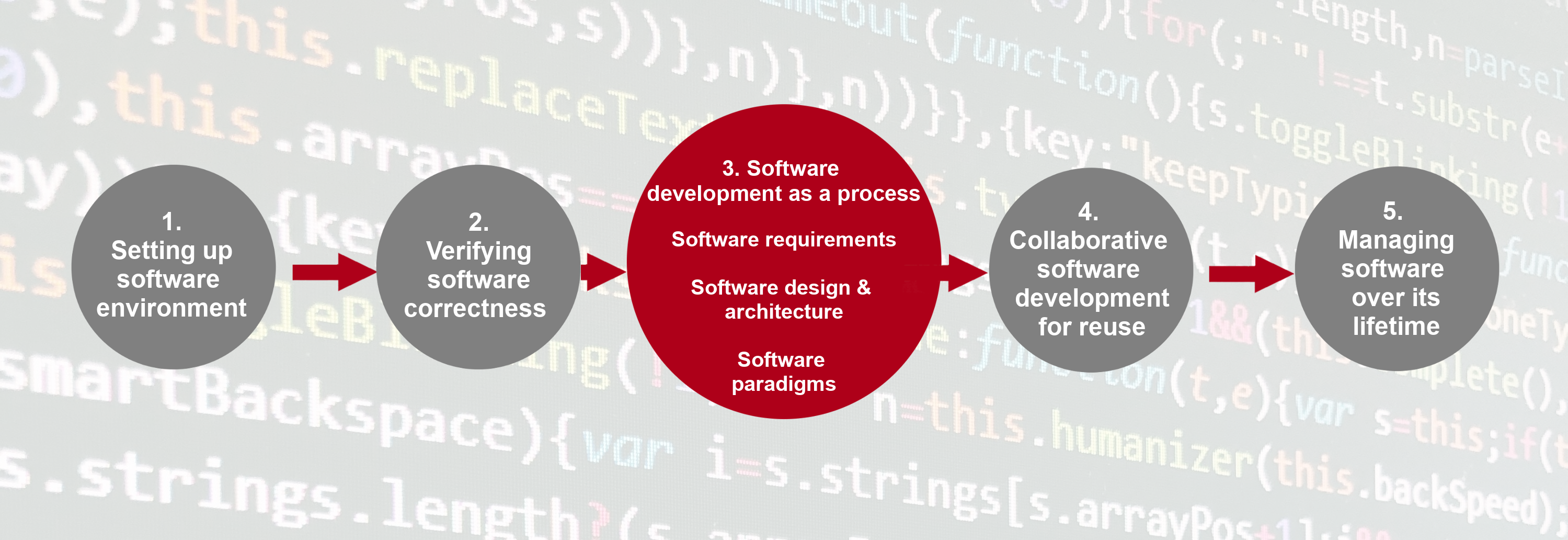
Writing Code vs Engineering Software
Traditionally in academia, software - and the process of writing it - is often seen as a necessary but throwaway artefact in research. For example, there may be research questions for a given research project, code is created to answer those questions, the code is run over some data and analysed, and finally a publication is written based on those results. These steps are often taken informally.
The terms programming (or even coding) and software engineering are often used interchangeably. They are not. Programmers or coders tend to focus on one part of software development: implementation, more than any other. In academic research, often they are writing software for themselves, where they are their own stakeholders. And ideally, they write software from a design, that fulfils a research goal to publish research papers.
Someone who is engineering software takes a wider view:
- The lifecycle of software: recognises that software development is a process that proceeds from understanding what is needed, to writing the software and using/releasing it, to what happens afterwards.
- Who will (or may) be involved: software is written for stakeholders. This may only be the researcher initially, but there is an understanding that others may become involved later (even if that isn’t evident yet). A good rule of thumb is to always assume that code will be read and used by others later on, which includes yourself!
- Software (or code) is an asset: software inherently contains value - for example, in terms of what it can do, the lessons learned throughout its development, and as an implementation of a research approach (i.e. a particular research algorithm, process, or technical approach).
- As an asset, it could be reused: again, it may not be evident initially that the software will have use beyond its initial purpose or project, but there is an assumption that the software - or even just a part of it - could be reused in the future.
The Software Development Process
The typical stages of a software development process can be categorised as follows:
- Requirements gathering: the process of identifying and recording the exact requirements for a software project before it begins. This helps maintain a clear direction throughout development, and sets clear targets for what the software needs to do.
- Design: where the requirements are translated into an overall design for the software. It covers what will be the basic software ‘components’ and how they’ll fit together, as well as the tools and technologies that will be used, which will together address the requirements identified in the first stage.
- Implementation: the software is developed according to the design, implementing the solution that meets the requirements set out in the requirements gathering stage.
- Testing: the software is tested with the intent to discover and rectify any defects, and also to ensure that the software meets its defined requirements, i.e. does it actually do what it should do reliably?
- Deployment: where the software is deployed or in some way released, and used for its intended purpose within its intended environment.
- Maintenance: where updates are made to the software to ensure it remains fit for purpose, which typically involves fixing any further discovered issues and evolving it to meet new or changing requirements.
The process of following these stages, particularly when undertaken in this order, is referred to as the waterfall model of software development: each stage’s outputs flow into the next stage sequentially.
Whether projects or people that develop software are aware of them or not, these stages are followed implicitly or explicitly in every software project. What is required for a project (during requirements gathering) is always considered, for example, even if it isn’t explored sufficiently or well understood.
Following a process of development offers some major benefits:
- Stage gating: a quality gate at the end of each stage, where stakeholders review the stage’s outcomes to decide if that stage has completed successfully before proceeding to the next one (and even if the next stage is not warranted at all - for example, it may be discovered during requirements of design that development of the software isn’t practical or even required).
- Predictability: each stage is given attention in a logical sequence; the next stage should not begin until prior stages have completed. Returning to a prior stage is possible and may be needed, but may prove expensive, particularly if an implementation has already been attempted. However, at least this is an explicit and planned action.
- Transparency: essentially, each stage generates output(s) into subsequent stages, which presents opportunities for them to be published as part of an open development process.
- It saves time: a well-known result from empirical software engineering studies is that it becomes exponentially more expensive to fix mistakes in future stages. For example, if a mistake takes 1 hour to fix in requirements, it may take 5 times that during design, and perhaps as much as 20 times that to fix if discovered during testing.
In this section we will place the actual writing of software (implementation) within the context of the typical software development process:
- Explore the importance of software requirements, the different classes of requirements, and how we can interpret and capture them.
- How requirements inform and drive the design of software, the importance, role, and examples of software architecture, and the ways we can describe a software design.
- Implementation choices in terms of programming paradigms, looking at procedural, functional, and object oriented paradigms of development. Modern software will often contain instances of multiple paradigms, so it is worthwhile being familiar with them and knowing when to switch in order to make better code.
- How you can (and should) assess and update a software’s architecture when requirements change and complexity increases - is the architecture still fit for purpose, or are modifications and extensions becoming increasingly difficult to make?
Key Points
Software engineering takes a wider view of software development beyond programming (or coding).
Ensuring requirements are sufficiently captured is critical to the success of any project.
Following a process makes development predictable, can save time, and helps ensure each stage of development is given sufficient consideration before proceeding to the next.
Programming Paradigms
Overview
Teaching: 10 min
Exercises: 0 minQuestions
How does the structure of a problem affect the structure of our code?
How can we use common software paradigms to improve the quality of our software?
Objectives
Describe some of the major software paradigms we can use to classify programming languages.
Introduction
As you become more experienced in software development it becomes increasingly important to understand the wider landscape in which you operate, particularly in terms of the software decisions the people around you made and why? Today, there are a multitude of different programming languages, with each supporting at least one way to approach a problem and structure your code. In many cases, particularly with modern languages, a single language can allow many different structural approaches within your code.
One way to categorise these structural approaches is into paradigms. Each paradigm represents a slightly different way of thinking about and structuring our code and each has certain strengths and weaknesses when used to solve particular types of problems. Once your software begins to get more complex it’s common to use aspects of different paradigms to handle different subtasks. Because of this, it’s useful to know about the major paradigms, so you can recognise where it might be useful to switch.
There are two major families that we can group the common programming paradigms into: Imperative and Declarative. An imperative program uses statements that change the program’s state - it consists of commands for the computer to perform and focuses on describing how a program operates step by step. A declarative program expresses the logic of a computation to describe what should be accomplished rather than describing its control flow as a sequence steps.
We will look into three major paradigms from the imperative and declarative families that may be useful to you - Procedural Programming, Functional Programming and Object-Oriented Programming. Note, however, that most of the languages can be used with multiple paradigms, and it is common to see multiple paradigms within a single program - so this classification of programming languages based on the paradigm they use isn’t as strict.
Procedural Programming
Procedural Programming comes from a family of paradigms known as the Imperative Family. With paradigms in this family, we can think of our code as the instructions for processing data.
Procedural Programming is probably the style you’re most familiar with and the one we used up to this point, where we group code into procedures performing a single task, with exactly one entry and one exit point. In most modern languages we call these functions, instead of procedures - so if you’re grouping your code into functions, this might be the paradigm you’re using. By grouping code like this, we make it easier to reason about the overall structure, since we should be able to tell roughly what a function does just by looking at its name. These functions are also much easier to reuse than code outside of functions, since we can call them from any part of our program.
So far we have been using this technique in our code - it contains a list of instructions that execute one after the other starting from the top. This is an appropriate choice for smaller scripts and software that we’re writing just for a single use. Aside from smaller scripts, Procedural Programming is also commonly seen in code focused on high performance, with relatively simple data structures, such as in High Performance Computing (HPC). These programs tend to be written in C (which doesn’t support Object Oriented Programming) or Fortran (which didn’t until recently). HPC code is also often written in C++, but C++ code would more commonly follow an Object Oriented style, though it may have procedural sections.
Note that you may sometimes hear people refer to this paradigm as “functional programming” to contrast it with Object Oriented Programming, because it uses functions rather than objects, but this is incorrect. Functional Programming is a separate paradigm that places much stronger constraints on the behaviour of a function and structures the code differently as we’ll see soon.
Functional Programming
Functional Programming comes from a different family of paradigms - known as the Declarative Family. The Declarative Family is a distinct set of paradigms which have a different outlook on what a program is - here code describes what data processing should happen. What we really care about here is the outcome - how this is achieved is less important.
Functional Programming is built around a more strict definition of the term function borrowed from mathematics. A function in this context can be thought of as a mapping that transforms its input data into output data. Anything a function does other than produce an output is known as a side effect and should be avoided wherever possible.
Being strict about this definition allows us to break down the distinction between code and data, for example by writing a function which accepts and transforms other functions - in Functional Programming code is data.
The most common application of Functional Programming in research is in data processing, especially when handling Big Data. One popular definition of Big Data is data which is too large to fit in the memory of a single computer, with a single dataset sometimes being multiple terabytes or larger. With datasets like this, we can’t move the data around easily, so we often want to send our code to where the data is instead. By writing our code in a functional style, we also gain the ability to run many operations in parallel as it’s guaranteed that each operation won’t interact with any of the others - this is essential if we want to process this much data in a reasonable amount of time.
Object Oriented Programming
Object Oriented Programming focuses on the specific characteristics of each object and what each object can do. An object has two fundamental parts - properties (characteristics) and behaviours. In Object Oriented Programming, we first think about the data and the things that we’re modelling - and represent these by objects.
For example, if we’re writing a simulation for our chemistry research, we’re probably going to need to represent atoms and molecules. Each of these has a set of properties which we need to know about in order for our code to perform the tasks we want - in this case, for example, we often need to know the mass and electric charge of each atom. So with Object Oriented Programming, we’ll have some object structure which represents an atom and all of its properties, another structure to represent a molecule, and a relationship between the two (a molecule contains atoms). This structure also provides a way for us to associate code with an object, representing any behaviours it may have. In our chemistry example, this could be our code for calculating the force between a pair of atoms.
Most people would classify Object Oriented Programming as an extension of the Imperative family of languages (with the extra feature being the objects), but others disagree.
So Which one is Python?
Python is a multi-paradigm and multi-purpose programming language. You can use it as a procedural language and you can use it in a more object oriented way. It does tend to land more on the object oriented side as all its core data types (strings, integers, floats, booleans, lists, sets, arrays, tuples, dictionaries, files) as well as functions, modules and classes are objects.
Since functions in Python are also objects that can be passed around like any other object, Python is also well suited to functional programming. One of the most popular Python libraries for data manipulation, Pandas (built on top of NumPy), supports a functional programming style as most of its functions on data are not changing the data (no side effects) but producing a new data to reflect the result of the function.
Other Paradigms
The three paradigms introduced here are some of the most common, but there are many others which may be useful for addressing specific classes of problem - for much more information see the Wikipedia’s page on programming paradigms. Having mainly used Procedural Programming so far, we will now have a closer look at Functional and Object Oriented Programming paradigms and how they can affect our architectural design choices.
Key Points
A software paradigm describes a way of structuring or reasoning about code.
Different programming languages are suited to different paradigms.
Different paradigms are suited to solving different classes of problems.
A single piece of software will often contain instances of multiple paradigms.
Functional Programming
Overview
Teaching: 30 min
Exercises: 30 minQuestions
What is functional programming?
Which situations/problems is functional programming well suited for?
Objectives
Describe the core concepts that define the functional programming paradigm
Describe the main characteristics of code that is written in functional programming style
Learn how to generate and process data collections efficiently using MapReduce and Python’s comprehensions
Introduction
Functional programming is a programming paradigm where
programs are constructed by applying and composing/chaining functions.
Functional programming is based on the
mathematical definition of a function
f(),
which applies a transformation to some input data giving us some other data as a result
(i.e. a mapping from input x to output f(x)).
Thus, a program written in a functional style becomes a series of transformations on data
which are performed to produce a desired output.
Each function (transformation) taken by itself is simple and straightforward to understand;
complexity is handled by composing functions in various ways.
Often when we use the term function we are referring to a construct containing a block of code which performs a particular task and can be reused. We have already seen this in procedural programming - so how are functions in functional programming different? The key difference is that functional programming is focussed on what transformations are done to the data, rather than how these transformations are performed (i.e. a detailed sequence of steps which update the state of the code to reach a desired state). Let’s compare and contrast examples of these two programming paradigms.
Functional vs Procedural Programming
The following two code examples implement the calculation of a factorial
in procedural and functional styles, respectively.
Recall that the factorial of a number n (denoted by n!) is calculated as
the product of integer numbers from 1 to n.
The first example provides a procedural style factorial function.
def factorial(n):
    """Calculate the factorial of a given number.

    :param int n: The factorial to calculate
    :return: The resultant factorial
    """
    if n < 0:
        raise ValueError('Only use non-negative integers.')

    factorial = 1
    for i in range(1, n + 1): # iterate from 1 to n
        # save intermediate value to use in the next iteration
        factorial = factorial * i

    return factorial
Functions in procedural programming are procedures that describe a detailed list of instructions to tell the computer what to do step by step and how to change the state of the program and advance towards the result. They often use iteration to repeat a series of steps. Functional programming, on the other hand, typically uses recursion - an ability of a function to call/repeat itself until a particular condition is reached. Let’s see how it is used in the functional programming example below to achieve a similar effect to that of iteration in procedural programming.
# Functional style factorial function
def factorial(n):
    """Calculate the factorial of a given number.

    :param int n: The factorial to calculate
    :return: The resultant factorial
    """
    if n < 0:
        raise ValueError('Only use non-negative integers.')

    if n == 0 or n == 1:
        return 1 # exit from recursion, prevents infinite loops
    else:
        return  n * factorial(n-1) # recursive call to the same function
Note: You may have noticed that both functions in the above code examples have the same signature (i.e. they take an integer number as input and return its factorial as output). You could easily swap these equivalent implementations without changing the way that the function is invoked. Remember, a single piece of software may well contain instances of multiple programming paradigms - including procedural, functional and object-oriented - it is up to you to decide which one to use and when to switch based on the problem at hand and your personal coding style.
Functional computations only rely on the values that are provided as inputs to a function and not on the state of the program that precedes the function call. They do not modify data that exists outside the current function, including the input data - this property is referred to as the immutability of data. This means that such functions do not create any side effects, i.e. do not perform any action that affects anything other than the value they return. For example: printing text, writing to a file, modifying the value of an input argument, or changing the value of a global variable. Functions without side affects that return the same data each time the same input arguments are provided are called pure functions.
Exercise: Pure Functions
Which of these functions are pure? If you’re not sure, explain your reasoning to someone else, do they agree?
def add_one(x):
    return x + 1

def say_hello(name):
    print('Hello', name)

def append_item_1(a_list, item):
    a_list += [item]
    return a_list

def append_item_2(a_list, item):
    result = a_list + [item]
    return result
Solution
add_oneis pure - it has no effects other than to return a value and this value will always be the same when given the same inputssay_hellois not pure - printing text counts as a side effect, even though it is the clear purpose of the functionappend_item_1is not pure - the argumenta_listgets modified as a side effect - try this yourself to prove itappend_item_2is pure - the result is a new variable, so this timea_listdoes not get modified - again, try this yourself
Benefits of Functional Code
There are a few benefits we get when working with pure functions:
- Testability
- Composability
- Parallelisability
Testability indicates how easy it is to test the function - usually meaning unit tests. It is much easier to test a function if we can be certain that a particular input will always produce the same output. If a function we are testing might have different results each time it runs (e.g. a function that generates random numbers drawn from a normal distribution), we need to come up with a new way to test it. Similarly, it can be more difficult to test a function with side effects as it is not always obvious what the side effects will be, or how to measure them.
Composability refers to the ability to make a new function from a chain of other functions
by piping the output of one as the input to the next.
If a function does not have side effects or non-deterministic behaviour,
then all of its behaviour is reflected in the value it returns.
As a consequence of this, any chain of combined pure functions is itself pure,
so we keep all these benefits when we are combining functions into a larger program.
As an example of this, we could make a function called add_two,
using the add_one function we already have.
def add_two(x):
    return add_one(add_one(x))
Parallelisability is the ability for operations to be performed at the same time (independently). If we know that a function is fully pure and we have got a lot of data, we can often improve performance by splitting data and distributing the computation across multiple processors. The output of a pure function depends only on its input, so we will get the right result regardless of when or where the code runs.
Everything in Moderation
Despite the benefits that pure functions can bring, we should not be trying to use them everywhere. Any software we write needs to interact with the rest of the world somehow, which requires side effects. With pure functions you cannot read any input, write any output, or interact with the rest of the world in any way, so we cannot usually write useful software using just pure functions. Python programs or libraries written in functional style will usually not be as extreme as to completely avoid reading input, writing output, updating the state of internal local variables, etc.; instead, they will provide a functional-appearing interface but may use non-functional features internally. An example of this is the Pandas library that we already used in previous episodes - most of its functions appear pure as they return new data objects instead of changing existing ones.
There are other advantageous properties that can be derived from the functional approach to coding. In languages which support functional programming, a function is a first-class object like any other object - not only can you compose/chain functions together, but functions can be used as inputs to, passed around or returned as results from other functions (remember, in functional programming code is data). This is why functional programming is suitable for processing data efficiently - in particular in the world of Big Data, where code is much smaller than the data, sending the code to where data is located is cheaper and faster than the other way round. Let’s see how we can do data processing using functional programming.
MapReduce Data Processing Approach
When working with data you will often find that you need to apply a transformation to each datapoint of a dataset and then perform some aggregation across the whole dataset. One instance of this data processing approach is known as MapReduce. This term usually arises in application to Big Data distributed processing on a cluster, e.g. using tools such as Spark or Hadoop. However, the name itself comes from applying an operation to (mapping) each value in a dataset, then performing a reduction operation which collects/aggregates all the individual results together to produce a single result. This approach can be modelled even on a single processor and a small dataset. MapReduce relies heavily on composability and parallelisability of functional programming - both map and reduce can be done in parallel and on smaller subsets of data, before aggregating all intermediate results into the final result.
Mapping
map(f, C) is a function takes another function f() and a collection C of data items as inputs.
Calling map(f, L) applies the function f(x) to every data item x in a collection C
and returns the resulting values as a new collection of the same size.
This is a simple mapping that takes a list of names and
returns a list of the lengths of those names using the built-in function len():
name_lengths = map(len, ["Mary", "Isla", "Sam"])
print(list(name_lengths))
[4, 4, 3]
This is a mapping that squares every number in the passed collection using anonymous, inlined lambda expression (a simple one-line mathematical expression representing a function):
squares = map(lambda x: x * x, [0, 1, 2, 3, 4])
print(list(squares))
[0, 1, 4, 9, 16]
Lambda
Lambda expressions are used to create anonymous functions that can be used to write more compact programs by inlining function code. A lambda expression takes any number of input parameters and creates an anonymous function that returns the value of the expression. So, we can use the short, one-line
lambda x, y, z, ...: expressioncode instead of defining and calling a named functionf()as follows:def f(x, y, z, ...): return expressionThe major distinction between lambda functions and ‘normal’ functions is that lambdas do not have names. We could give a name to a lambda expression if we really wanted to - but at that point we should be using a ‘normal’ Python function instead.
# Don't do this
add_one = lambda x: x + 1

# Do this instead
def add_one(x):
  return x + 1
In addition to using built-in or inlining anonymous lambda functions,
we can also pass a named function that we have defined ourselves to the map() function.
def add_one(num):
    return num + 1

result = map(add_one, [0, 1, 2])
print(list(result))
[1, 2, 3]
Exercise: Use Pandas Map and Apply functions for processing complex data
For common tasks, like filtering the table following a certain condition or applying arithmetical operations to table columns, with libraries like
numpyandpandasit is always better to use built-in functions, since they are often optimized and work much faster than usingmapwith a lambda function. However, not all data can be processed using already existing solutions. Apart from the Python built-inmapfunction,numpyandpandashave their own implementations of mapping, optimized for processing numpy arrays, Series and DataFrames. One situation in which it can be really handy is when you have a table with complex data stored in the columns, e.g. lists, dicts or arrays. For example, some surveys use such a format for storing light curves or spectra measurements. Let’s simulate such situation:# Create an empty list where we will be storing our light curves lcs = [] # For each observed object for obj_id in lc_datasets["lsst"]["objectId"].unique(): # Create an empty dict for the light curves of this object lc = {} lc['objectId'] = obj_id for b in bands: filt_band_obj = (lc_datasets["lsst"]["objectId"] == obj_id) & ( lc_datasets["lsst"]["band"] == b ) # The observations in each band are converted to lists and stored as dict elements lc[b+'_'+mag_col] = np.array(lc_datasets["lsst"][filt_band_obj][mag_col]) lc[b+'_'+time_col] = np.array(lc_datasets["lsst"][filt_band_obj][time_col]) lcs.append(lc) # Turn the list of dicts into a DataFrame lcs = pd.DataFrame.from_records(lcs)In the resulting DataFrame each row will contain an Id of the observed object, six columns for magnitude arrays and six corresponding columns with time stamps arrays. How would you deal with NaNs in the data stored in this format? For this task, you may find to be useful functions
pd.map,pd.apply,np.whereandnp.isnan. Try to come up with a solution where you replace the NaN values with zeros, and with a solution where you discard them entirely (don’t forget to remove the corresponding time stamps values too!).Solution
Let’s consider two possible solutions: the one where we replace the NaN values with zeros, and the one where we discard NaN values entirely. For the first solution we can use
pd.mapfunction, that act similarly to the classic Pythonmap, but works only forpd.Series.b = 'u' lcs[b+'_'+mag_col+'_cleaned'] = lcs[b+'_'+mag_col].map(lambda l: np.where(np.isnan(l),0,l))For the second solution, we need to remove not only NaN values from the magnitude arrays, but also corresponding to them time stamps. For this reason, we cannot use
pd.mapas it can be used only withpd.Series(e.g. with only one column). However, another Pandas function,apply, can accept rows.b = "u" # Create column names variables for better readability mcol = b + "_" + mag_col tcol = b + "_" + time_col mcol_cl = mcol + "_cleaned" tcol_cl = tcol + "_cleaned" # The new cleaned columns, `mcol_cl` and `tcol_cl`, contain the result of applying # a lambda function to each row (`axis=1` argument). The lambda function returns a tuple # of two numpy arrays, filtered according to the mask that is `False` for the elements that # are NaNs and `True` to all other elements. lcs[[mcol_cl, tcol_cl]] = lcs.apply( lambda l: ( l[mcol][~np.isnan(l[mcol])], l[tcol][~np.isnan(l[mcol])], ), axis=1, result_type="expand", )Note: you’re better not to store a table with any kinds of collections (lists, tuples, dictionaries or arrays) in the columns in a ‘.csv’ file, since reading and parsing it correctly can take a lot of effort.
Comprehensions for Mapping/Data Generation
Another way you can generate new collections of data from existing collections in Python is
using comprehensions,
which are an elegant and concise way of creating data from
iterable objects using for loops.
While not a pure functional concept,
comprehensions provide data generation functionality
and can be used to achieve the same effect as the built-in “pure functional” function map().
They are commonly used and actually recommended as a replacement of map() in modern Python.
Let’s have a look at some examples.
integers = range(5)
double_ints = [2 * i for i in integers]

print(double_ints)
[0, 2, 4, 6, 8]
The above example uses a list comprehension to double each number in a sequence. Notice the similarity between the syntax for a list comprehension and a for loop - in effect, this is a for loop compressed into a single line. In this simple case, the code above is equivalent to using a map operation on a sequence, as shown below:
integers = range(5)
double_ints = map(lambda i: 2 * i, integers)
print(list(double_ints))
[0, 2, 4, 6, 8]
We can also use list comprehensions to filter data, by adding the filter condition to the end:
double_even_ints = [2 * i for i in integers if i % 2 == 0]
print(double_even_ints)
[0, 4, 8]
Set and Dictionary Comprehensions and Generators
We also have set comprehensions and dictionary comprehensions, which look similar to list comprehensions but use the set literal and dictionary literal syntax, respectively.
double_even_int_set = {2 * i for i in integers if i % 2 == 0}
print(double_even_int_set)

double_even_int_dict = {i: 2 * i for i in integers if i % 2 == 0}
print(double_even_int_dict)
{0, 4, 8} {0: 0, 2: 4, 4: 8}Finally, there’s one last ‘comprehension’ in Python - a generator expression - a type of an iterable object which we can take values from and loop over, but does not actually compute any of the values until we need them. Iterable is the generic term for anything we can loop or iterate over - lists, sets and dictionaries are all iterables.
The
rangefunction is an example of a generator - if we created arange(1000000000), but didn’t iterate over it, we’d find that it takes almost no time to do. Creating a list containing a similar number of values would take much longer, and could be at risk of running out of memory.We can build our own generators using a generator expression. These look much like the comprehensions above, but act like a generator when we use them. Note the syntax difference for generator expressions - parenthesis are used in place of square or curly brackets.
doubles_generator = (2 * i for i in integers)
for x in doubles_generator:
   print(x)
0 2 4 6 8
Let’s now have a look at reducing the elements of a data collection into a single result.
Reducing
reduce(f, C, initialiser) function accepts a function f(),
a collection C of data items
and an optional initialiser,
and returns a single cumulative value which
aggregates (reduces) all the values from the collection into a single result.
The reduction function first applies the function f() to the first two values in the collection
(or to the initialiser, if present, and the first item from C).
Then for each remaining value in the collection,
it takes the result of the previous computation
and the next value from the collection as the new arguments to f()
until we have processed all of the data and reduced it to a single value.
For example, if collection C has 5 elements, the call reduce(f, C) calculates:
f(f(f(f(C[0], C[1]), C[2]), C[3]), C[4])
One example of reducing would be to calculate the product of a sequence of numbers.
from functools import reduce

sequence = [1, 2, 3, 4]

def product(a, b):
    return a * b

print(reduce(product, sequence))

# The same reduction using a lambda function
print(reduce((lambda a, b: a * b), sequence))
24
24
Note that reduce() is not a built-in function like map() -
you need to import it from library functools.
Exercise: Calculate the Sum of a Sequence of Numbers Using Reduce
Using reduce calculate the sum of a sequence of numbers. Although in practice we would use the built-in
sum()function for this - try doing it without it.Solution
from functools import reduce

sequence = [1, 2, 3, 4]

def add(a, b):
    return a + b

print(reduce(add, sequence))

# The same reduction using a lambda function
print(reduce((lambda a, b: a + b), sequence))
10 10
Putting It All Together
Let’s now put together what we have learned about map and reduce so far by writing a function that calculates the sum of the squares of the values in a list using the MapReduce approach.
from functools import reduce

def sum_of_squares(sequence):
    squares = [x * x for x in sequence]  # use list comprehension for mapping
    return reduce(lambda a, b: a + b, squares)
We should see the following behaviour when we use it:
print(sum_of_squares([0]))
print(sum_of_squares([1]))
print(sum_of_squares([1, 2, 3]))
print(sum_of_squares([-1]))
print(sum_of_squares([-1, -2, -3]))
0
1
14
1
14
Now let’s assume we’re reading in these numbers from an input file, so they arrive as a list of strings. We’ll modify the function so that it passes the following tests:
print(sum_of_squares(['1', '2', '3']))
print(sum_of_squares(['-1', '-2', '-3']))
14
14
The code may look like:
from functools import reduce

def sum_of_squares(sequence):
    integers = [int(x) for x in sequence]
    squares = [x * x for x in integers]
    return reduce(lambda a, b: a + b, squares)
Finally, like comments in Python, we’d like it to be possible for users to comment out numbers in the input file they give to our program. We’ll finally extend our function so that the following tests pass:
print(sum_of_squares(['1', '2', '3']))
print(sum_of_squares(['-1', '-2', '-3']))
print(sum_of_squares(['1', '2', '#100', '3']))
14
14
14
To do so, we may filter out certain elements and have:
from functools import reduce

def sum_of_squares(sequence):
    integers = [int(x) for x in sequence if x[0] != '#']
    squares = [x * x for x in integers]
    return reduce(lambda a, b: a + b, squares)
Decorators
Finally, we will look at one last aspect of Python where functional programming is coming handy. As we have seen in the episode on parametrising our unit tests, a decorator can take a function, modify/decorate it, then return the resulting function. This is possible because Python treats functions as first-class objects that can be passed around as normal data. Here, we discuss decorators in more detail and learn how to write our own. Let’s look at the following code for ways on how to “decorate” functions.
def with_logging(func):

    """A decorator which adds logging to a function."""
    def inner(*args, **kwargs):
        print("Before function call")
        result = func(*args, **kwargs)
        print("After function call")
        return result

    return inner


def add_one(n):
    print("Adding one")
    return n + 1

# Redefine function add_one by wrapping it within with_logging function
add_one = with_logging(add_one)

# Another way to redefine a function - using a decorator
@with_logging
def add_two(n):
    print("Adding two")
    return n + 2

print(add_one(1))
print(add_two(1))
Before function call
Adding one
After function call
2
Before function call
Adding two
After function call
3
In this example, we see a decorator (with_logging)
and two different syntaxes for applying the decorator to a function.
The decorator is implemented here as a function which encloses another function.
Because the inner function (inner()) calls the function being decorated (func())
and returns its result,
it still behaves like this original function.
Part of this is the use of *args and **kwargs -
these allow our decorated function to accept any arguments or keyword arguments
and pass them directly to the function being decorated.
Our decorator in this case does not need to modify any of the arguments,
so we do not need to know what they are.
Any additional behaviour we want to add as part of our decorated function,
we can put before or after the call to the original function.
Here we print some text both before and after the decorated function,
to show the order in which events happen.
We also see in this example the two different ways in which a decorator can be applied.
The first of these is to use a normal function call (with_logging(add_one)),
where we then assign the resulting function back to a variable -
often using the original name of the function, so replacing it with the decorated version.
The second syntax is the one we have seen previously (@with_logging).
This syntax is equivalent to the previous one -
the result is that we have a decorated version of the function,
here with the name add_two.
Both of these syntaxes can be useful in different situations:
the @ syntax is more concise if we never need to use the un-decorated version,
while the function-call syntax gives us more flexibility -
we can continue to use the un-decorated function
if we make sure to give the decorated one a different name,
and can even make multiple decorated versions using different decorators.
Exercise: Measuring Performance Using Decorators
One small task you might find a useful case for a decorator is measuring the time taken to execute a particular function. This is an important part of performance profiling. While in the Jupyter Lab you can use cell magics for this task, in
.pyfile a decorator is a suitable replacement.Write a decorator which you can use to measure the execution time of the decorated function using the time.process_time_ns() function. There are several different timing functions each with slightly different use-cases, but we won’t worry about that here.
For the function to measure, you may wish to use this as an example:
def measure_me(n):
    total = 0
    for i in range(n):
        total += i * i

    return total
Solution
import time

def profile(func):
    def inner(*args, **kwargs):
        start = time.process_time_ns()
        result = func(*args, **kwargs)
        stop = time.process_time_ns()

        print("Took {0} seconds".format((stop - start) / 1e9))
        return result

    return inner

@profile
def measure_me(n):
    total = 0
    for i in range(n):
        total += i * i

    return total

print(measure_me(1000000))
Took 0.124199753 seconds 333332833333500000
Key Points
Functional programming is a programming paradigm where programs are constructed by applying and composing smaller and simple functions into more complex ones (which describe the flow of data within a program as a sequence of data transformations).
In functional programming, functions tend to be pure - they do not exhibit side-effects (by not affecting anything other than the value they return or anything outside a function). Functions can also be named, passed as arguments, and returned from other functions, just as any other data type.
MapReduce is an instance of a data generation and processing approach, in particular suited for functional programming and handling Big Data within parallel and distributed environments.
Python provides comprehensions for lists, dictionaries, sets and generators - a concise (if not strictly functional) way to generate new data from existing data collections while performing sophisticated mapping, filtering and conditional logic on original dataset’s members.
Object Oriented Programming
Overview
Teaching: 30 min
Exercises: 40 minQuestions
How can we use code to describe the structure of data?
How should the relationships between structures be described?
Objectives
Describe the core concepts that define the object oriented paradigm
Use classes to encapsulate data within a more complex program
Structure concepts within a program in terms of sets of behaviour
Identify different types of relationship between concepts within a program
Structure data within a program using these relationships
Introduction
Object oriented programming is a programming paradigm based on the concept of objects, which are data structures that contain (encapsulate) data and code. Data is encapsulated in the form of fields (attributes) of objects, while code is encapsulated in the form of procedures (methods) that manipulate objects’ attributes and define “behaviour” of objects. So, in object oriented programming, we first think about the data and the things that we’re modelling - and represent these by objects - rather than define the logic of the program, and code becomes a series of interactions between objects.
Structuring Data
One of the main difficulties we encounter when building more complex software is how to structure our data. So far, we’ve been processing data from a single source and with a simple tabular structure, but it would be useful to be able to combine data from a range of different sources and with more data than just an array of numbers.
data = pd.DataFrame(data = [[1., 2., 3.],
                            [4., 5., 6.]],
                    columns = list('abc'))
Using this data structure has the advantage of being able to use Pandas operations to process the data and Matplotlib to plot it, but often we need to have more structure than this. For example, we may need to attach more information about the object which light curve we analyse, such as cutout image of this source or its spectra.
In a way, we already encountered this problem when we needed to store light curves of a single object, but obtained in different bands. Our solution then was to use a dictionary where keys corresponded to the bands names, and values were the DataFrames with the measurements. Generally speaking, we can expand this solution by adding new elements with values of other data types. For example, we could write something like this:
lc = {}
...
lc['spectra'] = np.array([4,5,6])
Since Python distionaries can store elements of different types, there is nothing that would stop us from this. We can also make nested dictionaries, creating really complex data structures.
Then we can get lost in them.
Classes in Python
Using nested dictionaries and lists should work for some of the simpler cases where we need to handle structured data, but they get quite difficult to manage once the structure becomes a bit more complex. For this reason, in the object oriented paradigm, we use classes to help with managing this data and the operations we would want to perform on it. A class is a template (blueprint) for a structured piece of data, so when we create some data using a class, we can be certain that it has the same structure each time.
With our dictionaries we had in the examples befpre, we have no real guarantee that each dictionary has the same structure unless we check it manually. With a class, if an object is an instance of that class (i.e. it was made using that template), we know it will have the structure defined by that class. Different programming languages make slightly different guarantees about how strictly the structure will match, but in object oriented programming this is one of the core ideas - all objects derived from the same class must follow the same behaviour.
You may not have realised, but you should already be familiar with some of the classes that come bundled as part of Python, for example:
my_list = [1, 2, 3]
my_dict = {1: '1', 2: '2', 3: '3'}
my_set = {1, 2, 3}

print(type(my_list))
print(type(my_dict))
print(type(my_set))
<class 'list'>
<class 'dict'>
<class 'set'>
Lists, dictionaries and sets are a slightly special type of class, but they behave in much the same way as a class we might define ourselves:
- They each hold some data (attributes or state).
- They also provide some methods describing the behaviours of the data - what can the data do and what can we do to the data?
The behaviours we may have seen previously include:
- Lists can be appended to
- Lists can be indexed
- Lists can be sliced
- Key-value pairs can be added to dictionaries
- The value at a key can be looked up in a dictionary
- The union of two sets can be found (the set of values present in any of the sets)
- The intersection of two sets can be found (the set of values present in all of the sets)
Encapsulating Data
Let’s start with a minimal example of a class representing a variable object.
class Variable:
    def __init__(self, obj_id):
        self.obj_id = obj_id
        self.lc = {
                   'mjd': np.array([]),
                   'mag': np.array([])
                  }

star_obs = Variable(obj_id)
print(star_obs.obj_id)
1405624461041897445
Here we’ve defined a class with one method: __init__.
This method is the initialiser method,
which is responsible for setting up the initial values and structure of the data
inside a new instance of the class -
this is very similar to constructors in other languages,
so the term is often used in Python too.
The __init__ method is called every time we create a new instance of the class,
as in Variable(obj_id).
The argument self refers to the instance on which we are calling the method
and gets filled in automatically by Python -
we do not need to provide a value for this when we call the method.
Data encapsulated within our Variable class includes the object’s id, and a light curve dictionary, that contains a numpy array with timestamps and a numpy array with magnitude measurements. In the initialiser method, we set an object’s id to the value provided, and create the numpy arrays for observations (initially empty). Such data is also referred to as the attributes of a class and holds the current state of an instance of the class. Attributes are typically hidden (encapsulated) internal object details ensuring that access to data is protected from unintended changes. They are manipulated internally by the class, which, in addition, can expose certain functionality as public behavior of the class to allow other objects to interact with this class’ instances.
Encapsulating Behaviour
In addition to representing a piece of structured data (e.g. an object that has an id and the lists with timestamps and magnitude observations), a class can also provide a set of functions, or methods, which describe the behaviours of the data encapsulated in the instances of that class. To define the behaviour of a class we add functions which operate on the data the class contains. These functions are the member functions or methods.
Methods on classes are the same as normal functions,
except that they live inside a class and have an extra first parameter self.
Using the name self is not strictly necessary, but is a very strong convention -
it is extremely rare to see any other name chosen.
When we call a method on an object,
the value of self is automatically set to this object - hence the name.
As we saw with the __init__ method previously,
we do not need to explicitly provide a value for the self argument,
this is done for us by Python.
Let’s add another method on our Variable class that adds observations to a Variable instance.
class Variable:
    """A Variable class"""
    def __init__(self, obj_id):
        self.obj_id = obj_id
        self.lc = {
                   'mjd': np.array([]),
                   'mag': np.array([])
                  }

    def add_observations(self, mjds, mags, mag_errs=None):
        """
        Adds observations to the light curve.

        Args:
          mjds: A vector of Modified Julian Dates (x values).
          mags: A vector of luminosities (y values).
        """
        self.lc['mjd'] = np.array(mjds)
        self.lc['mag'] = np.array(mags)
        if mag_errs is not None:
          self.lc['mag_errs'] = np.array(mag_errs)

        return


obj_id = lc_datasets['lsst']['objectId'].unique()[7]
b = 'g'
filt_band_obj = (lc_datasets['lsst']['objectId'] == obj_id) & (
        lc_datasets['lsst']['band'] == b
    )
obj_obs = lc_datasets['lsst'][filt_band_obj]
star = Variable(obj_id)
star.add_observations(obj_obs[time_col],obj_obs[mag_col])
print(star)
print(star.lc)
<__main__.Variable object at 0x7fc0fb40a750>
{'mjd': array([60559.2973682, 59791.3473572, 60559.2978172, 61017.0665232,
       60281.1630512, 59840.2103322, 60560.2654012
...
Note also how we used mag_errs=None in the parameter list of the add_observations method,
then initialise it if the value is not None, i.e. if the user passed magnitude errors.
This is one of the common ways to handle an optional argument in Python,
so we’ll see this pattern quite a lot in real projects.
Class and Static Methods
Sometimes, the function we’re writing doesn’t need access to any data belonging to a particular object. For these situations, we can instead use a class method or a static method. Class methods have access to the class that they’re a part of, and can access data on that class - but do not belong to a specific instance of that class, whereas static methods have access to neither the class nor its instances.
By convention, class methods use
clsas their first argument instead ofself- this is how we access the class and its data, just likeselfallows us to access the instance and its data. Static methods have neitherselfnorclsso the arguments look like a typical free function. These are the only common exceptions to usingselffor a method’s first argument.Both of these method types are created using decorators - for more information see the classmethod and staticmethod decorator sections of the Python documentation.
Dunder Methods
Why is the __init__ method not called init?
There are a few special method names that we can use
which Python will use to provide a few common behaviours,
each of which begins and ends with a double-underscore,
hence the name dunder method.
When writing your own Python classes,
you’ll almost always want to write an __init__ method,
but there are a few other common ones you might need sometimes.
You may have noticed in the code above that the method print(star)
returned <__main__.Patient object at 0x7fd7e61b73d0>,
which is the string representation of the star object.
We may want the print statement to display the object’s id instead.
We can achieve this by overriding the __str__ method of our class.
...
    def __str__(self):
      return str(self.obj_id)


star = Variable(obj_id')
print(star)
1405624461041897445
These dunder methods are not usually called directly,
but rather provide the implementation of some functionality we can use -
we didn’t call star.__str__(),
but it was called for us when we did print(star).
Some we see quite commonly are:
__str__- converts an object into its string representation, used when you callstr(object)orprint(object). Pay attention that we had to convert ourself.obj_idto string in order for this method to work__getitem__- Accesses an object by key, this is howlist[x]anddict[x]are implemented__len__- gets the length of an object when we uselen(object)- usually the number of items it contains
There are many more described in the Python documentation, but it’s also worth experimenting with built in Python objects to see which methods provide which behaviour. For a more complete list of these special methods, see the Special Method Names section of the Python documentation.
Exercise: Useful Methods for the Variable Class
Add several methods to our class, that would provide the following functionality:
- return the length of the lightcurve as the length of the
Variableinstance;- check that we are passing the suitable type of the data to our
add_observationsmethod, convert it intonp.arrayand check that the length of all observational arrays is the same.A hint: you may want to write several methods for the second task.
Solution
For the first task we can write our own
__len__dunder method:class Variable: ... def __len__(self): return len(self.lc["mjd"])For the second task we may want to break it into several features and write a function for each of them:
class Variable:
...

  def convert_to_array(self,data):
       # Check if the data is iterable and convert it into np.array, otherwise raise an exception
       if not isinstance(data, np.ndarray):
           if isinstance(data, (list,tuple,pd.Series)):
               data = np.array(data)
           elif isinstance(data, (int, float)):
               data = np.array([data])
           else:
               raise ValueError("The data type of the input is incorrect!")
       return data

   def compare_len(self,arrs):
       # Check that all arrays are of the same length
       lens = [len(arr) for arr in arrs]
       if len(set(lens)) > 1: # set() turns an iterable into a set of unique values.
       # If the values are all the same, the set will contain only one element
           raise ValueError("Passed timestamps and mags or mag_errs arrays have different lengths!")
       return

  def add_observations(self, mjds, mags, mag_errs=None):
       """
       Adds observations to the light curve.

       Args:
         mjds: A vector of Modified Julian Dates (x values).
         mags: A vector of luminosities (y values).
         mag_errs: A vector of magnitude errors.
       """
       self.lc["mjd"] = self.convert_to_array(mjds)
       self.lc["mag"] = self.convert_to_array(mags)
       if mag_errs is not None:
           self.lc["mag_errs"] = self.convert_to_array(mag_errs)
       self.compare_len(self.lc.values())
       return
Properties
The final special type of method we will introduce is a property. Properties are methods which behave like data - when we want to access them, we do not need to use brackets to call the method manually.
class Variable:
    ...

    @property
    def mean_mag(self):
        return np.mean(self.lc['mags'])
...
star = Variable(obj_id)
...
mean_mag = star.mean_mag
print(mean_mag)
18.03180312045771
You may recognise the @ syntax from episodes on
parameterising unit tests and functional programming -
property is another example of a decorator.
In this case the property decorator is taking the last_observation function
and modifying its behaviour,
so it can be accessed as if it were a normal attribute.
It is also possible to make your own decorators, but we won’t cover it here.
Relationships Between Classes
We now have a language construct for grouping data and behaviour related to a single conceptual object. The next step we need to take is to describe the relationships between the concepts in our code.
There are two fundamental types of relationship between objects which we need to be able to describe:
- Ownership - x has a y - this is composition
- Identity - x is a y - this is inheritance
Composition
In object oriented programming, we can make things components of other things.
We often use composition where we can say ‘x has a y’ -
for example in our lcanalyzer project,
we might want to say that a star has a multiband lightcurve,
or that a lightcurve has a single-band lightcurve.
In the case of our example, we’re already saying that our variable star has a lightcurve, so we’re already using composition here. We’re currently implementing a single-band lightcurve as a dictionary with a known set of keys though, and in the previous examples we used a dictionary to store DataFrames with single-band observations to represent multi-band data. Nothing stops us from turning these dictionaries into proper classes. In fact, this is exactly what we should do. For our current class example, it will look like this:
class Lightcurve:
    """Class Lightcurve"""
    def __init__(self, mjds=None, mags=None, mag_errs = None):
        self.lc = {}
        if mjds is not None:
            self.lc = self.add_observations(mjds, mags, mag_errs)

    def add_observations(self, mjds, mags, mag_errs = None):
        self.lc["mjds"] = self.convert_to_array(mjds)
        self.lc["mags"] = self.convert_to_array(mags)
        if mag_errs is not None:
            self.lc["mag_errs"] = self.convert_to_array(mag_errs)
        self.compare_len(self.lc.values())
        return self.lc

    def convert_to_array(self,data):
...

class Variable:
    """A Variable class"""

    def __init__(self, obj_id):
        self.obj_id = obj_id
        self.mband_lc = {}

    def add_lc(self,band,mjds,mags,mag_errs=None):
        self.mband_lc[band] = Lightcurve(mjds,mags,mag_errs)
        return self.mband_lc

    def __str__(self):
        return str(self.obj_id)


star = Variable(obj_id)
star.add_lc(band = b,mjds = obj_obs[time_col], mags = obj_obs[mag_col])
star.mband_lc['g'].mean_mag
18.03180312045771
Now we’re using a composition of two custom classes to
describe the relationship between two types of entity in the system that we’re modelling. The benefit of this
approach is that we can create a new class called e.g. Asteroid, and it will require implementing its own analysis methods that will
differ from those of the class Variable. The implementation of Asteroid class will be different, but it can
still have the Lightcurve. Note that this is only one possible implementation; for example, we are still storing
our light curve observations in a dictionary (self.lc = {}) to avoid rewriting our already existing functions,
but in reality it is likely will be more practical to turn mjds and mags into separate variables.
Inheritance
The other type of relationship used in object oriented programming is inheritance.
Inheritance is about data and behaviour shared by classes,
because they have some shared identity - ‘x is a y’.
If class X inherits from (is a) class Y,
we say that Y is the superclass or parent class of X,
or X is a subclass of Y.
Extending the previous example, we can recall that there are different types
of variables. For example, we can have periodic variables, such as RR Lyrae, or transient ones,
such as supernovae (or SNe for short). Periodic variables will need a method for
determining their periods, while transient ones will benefit from implementing
an algorithm for SNe classification. Instead of writing these
two classes completely independently, we can make them both the subclasses of the class Variable.
To write our class in Python,
we used the class keyword, the name of the class,
and then a block of the functions that belong to it.
If the class inherits from another class,
we include the parent class name in brackets.
class RRLyrae(Variable):
    """A class for RR Lyrae stars."""
    def __init__(self, obj_id):
        super().__init__(obj_id)
        self.period = None

    def period_determination(self, period_range=(0.1,3)):
        """A function to determine the period"""
        self.period = 0.3
        return

rr_lyrae = RRLyrae(obj_id)
rr_lyrae.period_determination()
print(rr_lyrae.mband_lc)
print(rr_lyrae.period)
{}
0.3
In this example, Variable is a parent class (or superclass),
and RRLyrae is a subclass.
There’s something else we need to add as well -
Python doesn’t automatically call the __init__ method on the parent class
if we provide a new __init__ for our subclass,
so we’ll need to call it ourselves.
This makes sure that everything that needs to be initialised on the parent class has been,
before we need to use it.
If we don’t define a new __init__ method for our subclass,
Python will look for one on the parent class and use it automatically.
This is true of all methods -
if we call a method which doesn’t exist directly on our class,
Python will search for it among the parent classes.
The order in which it does this search is known as the method resolution order.
The line super().__init__(obj_id) gets the parent class,
then calls the __init__ method,
providing the obj_id variable that Variable.__init__ requires.
This is quite a common pattern, particularly for __init__ methods,
where we need to make sure an object is initialised as a valid X,
before we can initialise it as a valid Y -
e.g. a valid Variable must have an obj_id,
before we can properly initialise a RRLyrae model with their data.
Composition vs Inheritance
When deciding how to implement a model of a particular system, you often have a choice of either composition or inheritance, where there is no obviously correct choice. For example, it’s not obvious whether a multi-messenger event (i.e. the one that has information coming with different carriers, such as electromagnetic waves and gravitational waves) is a light curve and is a chirp, or has a light curve and has a chirp.
class Observation:
    pass

class Lightcurve(Observation):
    pass

class Chirp(Observation):
    pass

class MultiMessengerEvent(Lightcurve, Chirp):
    # Multi-messenger event `is a` Lightcurve and `is a` Chirp
    pass
class Observation: pass class Lightcurve(Observation): pass class Chirp(Observation): pass class MultiMessengerEvent(Observation): def __init__(self): # Multi-messenger event `has a` Lightcurve and `has a` Chirp self.lc = Lightcurve() self.chirp = Chirp()Both of these would be perfectly valid models and would work for most purposes. However, unless there’s something about how you need to use the model which would benefit from using a model based on inheritance, it’s usually recommended to opt for composition over inheritance. This is a common design principle in the object oriented paradigm and is worth remembering, as it’s very common for people to overuse inheritance once they’ve been introduced to it.
For much more detail on this see the Python Design Patterns guide.
Multiple Inheritance
Multiple Inheritance is when a class inherits from more than one direct parent class. It exists in Python, but is often not present in other Object Oriented languages. Although this might seem useful, like in our inheritance-based model of the Multi-messenger event above, it’s best to avoid it unless you’re sure it’s the right thing to do, due to the complexity of the inheritance heirarchy. Often using multiple inheritance is a sign you should instead be using composition - again like the Multi-messenger event model above.
Key Points
Object oriented programming is a programming paradigm based on the concept of classes, which encapsulate data and code.
Classes allow us to organise data into distinct concepts.
By breaking down our data into classes, we can reason about the behaviour of parts of our data.
Relationships between concepts can be described using inheritance (is a) and composition (has a).
Software Requirements
Overview
Teaching: 15 min
Exercises: 20 minQuestions
Where do we start when beginning a new software project?
How can we capture and organise what is required for software to function as intended?
Objectives
Describe the different types of software requirements.
Explain the difference between functional and non-functional requirements.
Describe some of the different kinds of software and explain how the environment in which software is used constrains its design.
Up until now we treated our project as a collection of functional elements. We looked through it line by line to fix style errors and coding conventions, then we looked at separate functions to write unit tests, and then we analyzed its functions to find out how we can rewrite the code using OOP (Object Oriented Programming). However, designing software that will be both useful and maintainable over the long term means more than writing code that can perform certain tasks. There are a number of factors that we need to take into account, such as how fast the code needs to work, what kind of computational resources it will need, how easy it will be to add new functionality, how convenient it will be to the end user and so on.
It is not a trivial task to think about all these factors while writing the code, even for a small project, and it can be a great deal of work to add functionality retroactively if a piece of software is poorly designed. So it is much more reasonable to think about them in advance. The idea of separating the planning stage from the implementation stage led to the appearance of the concept of Software Development Life Cycle.
Software Development Life Cycle (SLDC)
Software Development Life Cycle (SLDC) is a methodology that splits the process of software development into a number of stages (usually between four and six):
- Requirements gathering and analysis: determining what functionality the stakeholders want. For large projects this stage includes user surveys and domain analysis (What functionality is already provided by pre-existing, similar projects? What are the unsolved problems of the potential users?). For a small project this step may be as short as writing down a list of desired features;
- Planning: determining what resources are needed to fulfill the requirements and deciding how the work process is going to be organized. For large projects it may include decisions to hire more people for the development team or obtaining more CPUs/GPUs for the cluster. For a small project it may be as short as deciding which Python libraries will be used;
- Software design: outlining software architecture. At this stage, the detailed description of how the software will be designed is produced, shared with the stakeholders and edited in accordance with the feedback;
- Development/Implementation: writing the code;
- Testing. This phase includes not only unit testing (which is normally done during the development stage, especially if Test-Driven Development is used), but also integration testing, performance testing, beta testing (manual) and so on;
- Deployment: installing the software in the operating environment (which can be very different from the development environment), familiarizing the end users with the software;
- Maintenance.
Each stage of SDLC is a separate discipline with its own practices, standards and documentation. Small teams, typical in science, often don’t have the resources to utilize these standards and methodologies. However, even a single-developer ‘team’ can benefit from using a simplified form of SLDC.
Life Cycle Models
Depending on the project, going through the SDLC stages only once and in sequential order is usually not the best idea. What if it becomes clear that you need additional functions after you implemented the first set of features, or if you need to adapt the software for a new operational environment - let’s say, migrate it into a cloud?
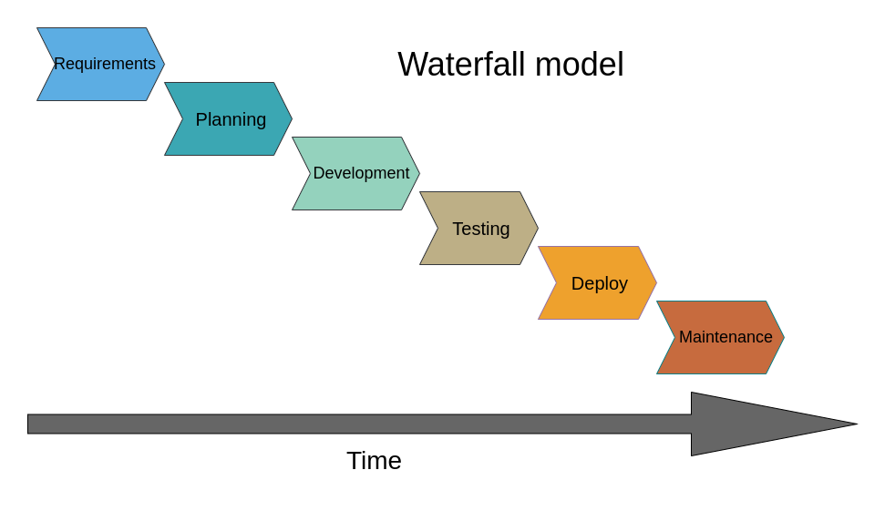
For such situations, different SDLC models exist. The sequential one, when all the stages follow one another only once, is called the Waterfall model, however, nowadays it’s not very common. The way software development is often done in academia, with little to no requirements analysis and planning before the development itself, is called the Big Bang model. While acceptable for short small-scale projects (or prototypes), sticking to this paradigm after the project exceeds a couple of hundred lines of code leads to chaos, computational ineffectiveness and poor maintainability.
What Comes After the Big Bang (Model)
In industry, one of the most popular SDLCs is Agile. This approach assumes that all stages of the life cycle are performed in iterations, or time-limited sprints (usually 1-4 weeks), with each sprint having a well-defined and relatively small goal (such as implementation of a single feature). This methodology aims to be flexible enough to incorporate requirements as they appear, and at the same time strict enough to not skip the requirements analysis altogether.
Let’s assume that you started writing the LCAnalyzer as a small script for a quick data exploration, but now new collaborators join your project, and they will need some additional functionality. In this situation we can treat our code as a prototype, developed following the Big Bang SDLC model, and we want to continue in a more organized fashion, using Agile-like approach. The first step is to gather requirements.
Prototype is for throwing it away
In case when the requirements aren’t clear from the beginning, starting with a prototype to figure them out is a perfectly valid choice. However, it is important to be ready to throw the prototype away and start again from scratch in case the discovered requirements and constraints reveal that originally chosen architecture is not the most suitable. It is hard to say at what point it’s time to switch from Big Bang-style prototyping to a more organized development methodology, but it’s a good idea to consider this after your code becomes larger than a hundred lines. The larger your prototype, the harder it is to admit that you have to put it aside and the longer it will take to create a new version with a different, more efficient architecture.
The first stage of SLDC: Requirements Gathering and Analysis
Software requirements are the answer to a question “what our software is supposed to do”. There is a hierarchy to them: they are usually separated into Business, User/Stakeholder and Solution Requirements.
Business requirements describe what is needed from the perspective of the organization, and define the strategic path of the project, e.g. to embark on a new research area or collaborative partnership. User/Stakeholder requirements define what particular stakeholder groups each expect from an eventual solution, essentially acting as a bridge between the higher-level business requirements and specific solution requirements. Finally, Solution (or product) requirements describe characteristics that software has to have in order to satisfy the stakeholder requirements.
The reasoning behind this hierarchy is that the answer to a question “what our software should do” will depend on who you ask. For example, a PI of a research group when writing a funding proposal will answer this question like this:
- BR 1: The software must extract periods for all periodic sources in an LSST Data Release within 2 weeks after the release is public.
Starting the development with this requirement alone will end in a huge disappointment, since formally you can deliver a package that will produce a table with two columns, an object ID and a period estimation, and it won’t be enough for a proper scientific analysis. At the same time, it is excellent for estimating the scope of the project: it states the main purpose of the software, what the input data will be and what are the computational constraints. Such a requirement can be considered as a business requirement.
A postdoc who’s going to use this software will give a different answer, somewhere along the lines of: “the software must determine the periods with three period-finding algorithms, and it must be able to plot phased light curves and periodograms”. This kind of answer gives us something to work with: at the very least we understand that we need to implement:
- UR 1.1: The software must be able to determine periods with Lomb-Scargle, binned means and SuperSmooth period-finding algorithms.
- UR 1.2: The software must be able to plot a phase-folded light curve.
- UR 1.3: The software must be able to plot a periodogram.
Each of these items is a User requirement.
Still, if we start the development with those requirements, we’ll encounter a number of uncertainties. For example, what should we do if our light curves contain NaNs or outlying data points? And should the software be able to plot folded light curves for all the millions of periodic sources in the LSST Data Release?
Such questions are answered with the lowest-level, or solution, requirements, which are split in two categories. The first one, functional requirements, correspond to the smallest features of the software. E.g. the software must drop NaNs and outlying values.
- SR 1.1.1: The software must drop NaNs and outlying values before running period finding algorithms.
-
SR 1.1.2: The software must read light curves in .csv, .pkl, .dat formats.
The second category is called non-functional requirements, and they define how these features will be implemented. They constrain things like computational performance, security or usability. E.g. if the user asks to plot more than 10 light curves, they must be saved as .png on a drive instead. Or, thinking about the original business requirement, we should specify that the software must be able to analyze a million sources in under three days.
- SR 1.1.3: The software must be able to determine periods for a million sources in under 3 days.
- SR 1.2.1: The software must be able to display plots on screen or save them as .png.
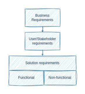
Not all requirements will be implemented.
In a perfect world, we would be able to implement all the desired requirements by the time we go to lunch. In reality, we have limited resources, and quite often we have to make sacrifices or risk never finishing the work at all.
After the requirements are written down, it is time to look over them and decide how realistic they are, considering available time and people resources. For this we can use a MoSCoW methodology. MoSCoW is an acronym that stands for Must have, Should have, Could have, and Won’t have, and each requirement, after a discussion with the stakeholders, falls into one of these four categories:
- Must Have (MH) - these requirements are critical to the current timebox for it to succeed. Even the inability to deliver just one of these would cause the project to be considered a failure.
- Should Have (SH) - these are important requirements but not necessary for delivery in the timebox. They may be as important as Must Haves, but there may be other ways to achieve them or perhaps they can be held back for a future development timebox.
- Could Have (CH) - these are desirable but not necessary, and each of these will be included in this timebox if it can be achieved.
- Won’t Have (WH) - these are agreed to be out of scope for this timebox, perhaps because they are the least important or not critical for this phase of development.
It is also common to plan a sprint in such a way that MH/SH/CH categories took 60%/20%/20% of working time correspondingly. This approach helps to ensure that SH and CH requirements aren’t neglected, and at the same provides enough time cushion to redistribute it if needed.
Collaborative work on requirements
Split in pairs and go into breakout rooms. Create a common Google Document. Imagine that you are a PI writing a funding proposal. Think for a few minutes and write down in the document a Business Requirement and subsequent Stakeholder requirements for some kind of software that would be useful in your work. Then take each other’s Business Requirements and write down several Solution requirements for this future software. When it’s done, provide each other with feedback on whether you think the Solution requirements will be enough for developing the software you need. Don’t forget about non-functional requirements, and don’t forget that not all requirements are realistic! If the Business Requirement includes ‘do a differential imaging on the whole LSST image dataset for 10 years in under 10 hours’, this part of the requirement has to be crossed out. If you are going through this materials on your own and don’t have a learning partner, you can use a new business requirement for the LCAnalyzer:
BR 2: The software must perform periodic/non-periodic classification of all variable sources in the LSST Data Release.
Solution
User requirements:
UR 2.1: The software must be able to calculate a reliability score of the found periods for each of the period-finding algorithms.
UR 2.2: The software must be able to calculate a probability that the source is variable based on the reliability scores for the obtained periods and on the closeness of the periods determined with different methods.
UR 2.3: For the sources for which no algorithm produces a reliable period, the software must run a transient event detection algorithm.
Solution requirements:
Functional:
SR 2.1.1: The software must calculate a reliability score of the period found by each of the implemented algorithms. The reliability score must vary from 0 to 1.
SR 2.2.1: The software must calculate two probability metrics relating to the variability of the source: one calculated as a median reliability score for the determined periods, and another as a mean deviation of the discovered periods.
SR 2.3.1: The software must run a transient event detection algorithm for the sources for which no periods were determined, or for which the probability of being variable is below a user-defined threshold.
Non-functional:
SR 2.3.2: The software must run a transient event detection algorithms in under 1 second per source.
From Requirements to Implementation, via Design
In practice, these different types of requirements are sometimes confused and conflated when different classes of stakeholders are discussing them, which is understandable: each group of stakeholders has a different view of what is required from a project. The key is to understand the stakeholder’s perspective as to how their requirements should be classified and interpreted, and for that to be made explicit. A related misconception is that each of these types are simply requirements specified at different levels of detail. At each level, not only are the perspectives different, but so are the nature of the objectives and the language used to describe them, since they each reflect the perspective and language of their stakeholder group.
It’s often tempting to go right ahead and implement requirements within existing software, but this neglects a crucial step: do these new requirements fit within our existing design, or does our design need to be revisited? It may not need any changes at all, but if it doesn’t fit logically our design will need a bigger rethink so the new requirement can be implemented in a sensible way. We’ll look at this a bit later in this section, but simply adding new code without considering how the design and implementation need to change at a high level can make our software increasingly messy and difficult to change in the future.
Key Points
When writing software used for research, the requirements will almost always change.
Consider non-functional requirements (how the software will behave) as well as functional requirements (what the software is supposed to do).
The environment in which users run our software has an effect on many design choices we might make.
Consider the expected longevity of any code before you write it.
Software Architecture and Design
Overview
Teaching: 15 min
Exercises: 20 minQuestions
What should we consider when designing software?
How to determine which components our software will have?
Objectives
Understand how software requirements are turned into software design.
Understand the main stages of software design.
Introduction
In this episode, we’ll be looking at how we can design our software to ensure it meets the requirements, but also retains the other qualities of good software. Software design, as opposed to software requirements, deals with how a project will be realized in terms of data structures, algorithms and system architecture. Requirements, on the other hand, specify what must be accomplished.
What is software architecture?
As soon as we know what our software is supposed to do, we have to find out how it will be doing what it’s doing. This is where software architecture comes into play. Software engineering borrowed this term, and a few other terms, from architects (of buildings) as many of the processes and techniques have some similarities. One of the other important terms we borrowed is ‘pattern’, such as in design patterns and architecture patterns. This term is often attributed to the book ‘A Pattern Language’ by Christopher Alexander et al. published in 1977 and refers to a template solution to a problem commonly encountered when building a system.
Design patterns are relatively small-scale templates which we can use to solve problems which affect a small part of our software. One example is a strategy pattern that could handle multiple algorithms and handling them in a consistent way. Architecture patterns are similar, but larger scale templates which operate at the level of whole programs, or collections or programs. Model-View-Controller is one of the best known architecture patterns. During the development process, programmers using the Python web framework Django will encounter it frequently.
Many patterns rely on concepts from Object Oriented Programming and there are many online sources of information about design and architecture patterns, often giving concrete examples of cases where they may be useful. One particularly good source is Refactoring Guru.
To determine software architecture means to describe which components (modules, classes, functions, databases) are going to be implemented, what are the relations between them, and how they are going to interact with each other, with other software and with the user. Software architecture leads the design and implementation of the software. To design the architecture of your software, several things have to be taken into account:
- Flexibility. What kind of additional functionality may be included in the future? What kind of architecture allows you to implement new features more easily?
- Performance/Scalability. What are the potential ‘bottlenecks’ of your software (e.g. a computationally-expensive calculation, or the necessity to download heavy observational data in real time)? Which architecture speeds up these slow parts of the software? (E.g. computationally-expensive calculations may be parallelized and performed on a cluster and its results sent back to your PC; instead of downloading large volumes of the data it may be possible to run the code where the data is stored, e.g. on Rubin Science Platform). If you develop software for multiple users, you need to consider if they’ll need simultaneous access to the same resources.
- Portability. Will this software be launched on other platforms, e.g. on an institute’s cluster or in a cloud?
- Maintainability. How simple is it going to be to test this software? Will its design be clear enough for other developers (e.g. your students) to troubleshoot it when needed?
- Security. If your software uses proprietary data, how data access rights will be preserved? If you are developing a server-based software for multiple users, how are you going to develop authorization?
- Integration with other software and user interfaces. What kind of data your software may need from other applications? What kind of outputs your software will produce, and will it be easy to implement a new output format or user interface (e.g. to create an interactive plot or store the calculation results in JSON instead of DAT)?
Similarly to the hierarchy of the requirements, the design process also has stages, with the next stage outlining smaller details than the previous one. This is the so called ‘top-down’ approach. For the large project this approach is more common and more efficient than ‘bottom-up’.
Software design process can be split into following phases:
- Component design. At this stage, the general blueprint of the software is created. Component design describes separate services, pipelines and modules, and then lists classes and stand-alone functions, together with a rough description on how they are going to interact with each other.
- Data design. At this stage it is determined which data structures will be used.
- Interface design. This stage is for determining public methods of the classes and finding out how different components will interact with each other.
- Procedural design. Here specific algorithms within the components are determined.
Software Design methods
There are several ways to go from the list of requirements to software architecture.
The noun-in-text. Write down a short description of the software, and then identify all nouns in the text. The nouns related to the environment outside of the software are thrown away, and those that mean the same concept are ‘merged’. The nouns that are related to the same concepts are grouped together, with one noun in the group being selected as the most representative of the group. This noun usually becomes a class, and the rest of the nouns in the group may become inherited classes or turn out to be good class attributes. This method is applicable even if you have only a general description of the software, so it’s suitable for working on a small project, and it’s especially helpful for the component design stage. It can also be applied to the user or solution requirements - or used for for writing them.
Exercise: The noun-in-text practice
Let’s say that we are starting a new project: we want to develop a package that detects faint structures on the galaxy images. We want the software to be able to read images in different formats and produces a list of detected structures. For each detected structure, the package should produce a corresponding image file that would indicate which pixels belong to the detected faint structure.
Using this description of software, apply noun-in-text approach to identify the main components of the software and decide which of the nouns will be classes, which will become attributes and which will be discarded. Think on the uncertainties that arise in the process and on the different possible architectures for this case.
Solution
The list of nouns will look like this: faint structures, galaxy, image, format, list of detected structures, detected structure, corresponding image file, pixel belonging to the structure
Without knowing anything about astronomy, we can presume that our software will have:
- class
Imagewith attributesstr: formatandGalaxy: galaxy;- class
Galaxywith attributelist: detected_structures;- and class
FaintStructurewith attributeimage: belonging_pixels.However, after some consideration it becomes apparent that there is a number of uncertainties. Does an image always contain one and only one galaxy, or there may be several galaxies in the image? Does the user pass the list of detected galaxies pictured in the image before launching faint structure detection, or do we need galaxy detection feature within the package as well? What are the properties of a detected galaxy - is it defined only by its center coordinates or it has a mask indicating which pixels belong to which galaxy? Is it possible for a faint structure to be detected without a host galaxy?
Answering these questions leads to new User and Solution requirements and will affect the design of the software.
Use case scenarios. Imagine a potential user of your software, then identify what will be the goal of this user, when running your software, and then write down the steps that the user will need to take in order to reach this goal. This method works well for the interface design stage, however, it is useful for component and data design too.
Using diagrams. There are various types of those; we will consider only two: system and class diagrams.
System diagram
System diagram is an overarching visualization of the major components of the system. It can demonstrate the data flow and use case scenarios, as well as connections to external resources. Creating such a diagram is useful for larger projects. Below a system diagram taken from the LSST Data Product Definition Document illustrates the conceptual design of the LSST pipelines for processing images.
System diagram of the conceptual design of LSST science pipelines for imaging processing. Without imposing any constraints on the implementation of the science pipelines, this diagram outlines that there will be eight major and largely independent pipelines, and gives information about which connections to the external databases are needed and which output catalogs will be produced at each stage.
Class diagram
For a more detailed design description, we can use a class diagram. It depictures classes together with their attributes, methods and relationships (such as composition or inheritance) using a set of conventions called Unified Modeling Language, or UML.
An example of object model diagrams of two possible implementations of the LCAnalyzer. These implementations have the same functionality, but different architectures. The first example has a single class ‘Dataset’, and its methods (listed in the bottom part of the box; the middle section contains class attributes) perform everything from reading the files to plotting periodograms. It doesn’t create a separate object ‘LightCurve’, but instead stores the data as a table (‘ndarray: data’). Extracting the necessary observational datapoints from the records of this table will be the responsibility of every function that will use them. This architecture is likely to produce a lot of duplicated code and will make adding new functionality difficult, however, it can be computationally effective, if many of the functions can be vectorised (effectively applied to a numeric array in which our light curves are stored). In the second architecture, we separate functionality related to the dataset as a whole from the features related to the light curves processing. Even more, every LightCurve object has a dictionary where observations in different bands are stored, with Observations being another class. Plotting functions are also put in a separate class and completely independent (there is no connector joining this class with the others), which means that we can use them even without having a DataLoader or LightCurve instance. This architecture is better in terms of separation of concerns, more convenient to test and more flexible.
Exercise: Developing class diagram for the Faint Structure Detection software
In this exercise you will use an online diagram drawing tool to create a class diagram for the faint structure detecting software from the previous exercise. Using this link, you can open a file with pre-defined blocks and turn them into a class diagram (the link opens a file on the Google Drive; in the drop-down menu on top of the window choose ‘Open with draw.io’). Feel free to move and create additional classes, attributes and methods as you see needed, and think how this architecture would work in practice. Some of the methods and attributes are intentionally placed into the wrong classes!
After doing that, let’s imagine that you realised that you have a new requirement for your software: The user should be able to manually draw a mask (to exclude bright stars, artefacts and so on) that will be applied before the stream detection. Look at your class diagram. Modify it to add the new feature. Do you encounter any difficulties? Did you have to rework a large part of the architecture to satisfy this new requirement?
Solution
One of the possible solutions is pictured below. Here we have three offered classes and one new class for plotting and drawing functions. Considering that classes “Galaxy” and “FaintStructure” are pretty similar up until now, we could also go with creating a parent class ‘Structure’ for which “Galaxy” and “FaintStructure” would be child classes.
There are multiple tools for drawing diagrams. You can use any of them, including diagram blocks in Google Docs or any other office application. And unless you need to prepare a public software documentation, you can even draw them by hand, if that’s more convenient. Time: 10 minutes
Software Requirements Document and Software Design Document
As was mentioned in the previous episode, each life cycle stage has its own best practices, specifications and formats. Two common types of specifications are Software Requirements Document (SRD) and Software Design Document (SDD):
- SRD focuses on ‘what’ the system does, describing its main purpose, potential users, their needs and expectations (often in the form of use case scenarios), the system’s necessary and desireable features. As the name suggests, it also includes full list of the requirements;
- SDD addresses how the system does it, including the architectural design, detailed components and data structures, diagrams, pseudocode, interface layouts, etc.
There are multiple templates of these types of documentation. The LSST Transient and Variable Sky Science Collaboration has its own astronomy-adapted SRD and SDD templates, written based on the IEEE recommendations and available for everyone. Hovewer, for a small-scale project it is acceptable to go with a simplified version of these documents, that boils down to a checklist:
SRD checklist:
- Introduction
- Purpose & Scope
- Audience/Stakeholders
- Problems within the scope of the software
- References, definitions, acronyms
- Overall Description
- Context (self-contained, part of larger family)
- Major functions as bullet points
- User classes and characteristics
- Where will the software be operated?
- Interface Requirements
- User interfaces
- Software and hardware interfaces
- Communication interfaces/protocols
- System Features
- Description and Priority
- Stimulus/Response (use case scenarios)
- Functional Requirements
- Nonfunctional Requirements
- Performance Requirements
- Security Requirements
SDD checklist:
- Software Overview
- Architecture Description
- Data flow diagram
- Dependencies
- Development Process
- Hardware design decisions
- Technology stack
- Coding standards & testing strategy
- Security & Backup
- Roadmap (work plan, timeline estimation)
- Possible future functionality
- Detailed description
- Components and their relationship
- Data Model
- Interface design (front-end, jupyter, API)
- Procedural design, e.g. diagram, pseudo-code
At what stage it’s time to start using these techniques?
Aspirationally, what makes good code can be summarised in the following quote from the Intent HG blog:
“Good code is written so that is readable, understandable, covered by automated tests, not overcomplicated and does well what is intended to do.”
By taking time to design our software to be easily modifiable and extensible, we can save ourselves a lot of time later when requirements change. The sooner we do this the better - ideally we should have at least a rough design sketched out for our software before we write a single line of code. This design should be based around the structure of the problem we’re trying to solve: what are the concepts we need to represent and what are the relationships between them. And importantly, who will be using our software and how will they interact with it?
How much effort should we spend on designing our code properly and using good development practices? The following XKCD comic summarises this tension:

There are a wealth of practices that could be used,
and this abundance can be intimidating. It is tempting
to skip the requirements analysis, planning and design stages and just go on with the
Big Bang SDLC model. However, picking one or two software design
approaches and using them at the beginning of every software project, even a small one,
is what separates an intermediate developer from someone who has just started coding.
It is much better to have a few use case scenarios written in a .txt file and a photo
of a class diagram drawn on a napkin from a cafeteria than to have an empty
fancy template of a Software Design Document and a thousand lines of spagetti-code
written with no preliminary architecture in mind. Make it a habit to spend
at least ten minutes writing down the requirements and software architecture
every time you open your IDE, and it will save you months of work in the future.
Key Points
Planning software projects in advance can save a lot of effort and reduce ‘technical debt’ later - even a partial plan is better than no plan at all.
By making our software modular, i.e. introducing parts with a single responsibility, we avoid having to rewrite it all when requirements change. Such components can be as small as a single function, or be a software package in their own right.
When writing software used for research, requirements will almost always change.
‘Good code is written so that is readable, understandable, covered by automated tests, not over complicated and does well what is intended to do.’
Architecture Revisited: Adding a .py Controller
Overview
Teaching: 15 min
Exercises: 50 minQuestions
How can we extend our software within the constraints of the MVC architecture?
Objectives
Extend our software to add a command line interface to request a specific view.
As we have seen, we have different programming paradigms that are suitable for different problems and affect the structure of our code. In programming languages that support multiple paradigms, such as Python, we have the luxury of using elements of different paradigms and we, as software designers and programmers, can decide how to use those elements in different architectural components of our software.
Now, let’s use what we’ve learned in the previous episodes and bring together software requirements, software design and actual development.
Exercise: A Survey Class
Use what we’ve learned to develop a class for processing the survey dataset itself. You already have most of the functionality implemented, now you have to think about how to re-implement it within an OOP paradigm. At the early stages of a software project it is pretty common to spend some time drafting out separate features before getting a cleare picture of what your software will be as a whole, especially if you work alone. This is called ‘bottom-up design’ (as opposed to the ‘top-down design’, in which you start with drafting the overall architecture). Create a new branck for this work (you can call it
dev-oopor something similar).We can start with defining the requirements. Let’s start with the following ones:
- SR1.1.1: the package can read the data in different formats, such as .csv and .pkl;
- SR1.1.2: the package can filter out the rows with NaN entries, where NaNs can be filled with different values (e.g. -99.9).
- SR1.1.3: the package can return the list of unique object IDs;
- SR1.1.4: the package can return a dict with the light curve of a user specified object in a user specified band.
Think of a few more, and write them on the top of you new notebook (or
.pyfile if that’s more convenient for you) before starting your work.Try using Test Driven Development for any features you add: write the tests first, then add the feature. Don’t forget to put the code you finished in the
.pyfiles!Solution
Let’s assume that in addition to the requirements above we also added two more functional requirements:
- SR1.1.5: the package can return a DataFrame with all the observations of a given object in a given band;
- SR1.1.6: the package can plot an unfolded light curve.
We can start the implementation with this:
- in the
lcanalyzerdirectory we can create two new files for the models level of our architecture:lightcurve.pywhich will contain theLightcurveclass, andsurvey.pythat will containe theSurveyclass. Also we will create a fileplots.pyfor the views level of the architecture.- in the
testsdirectory we will create filestest_lightcurve.py,test_survey.pyandtest_plots.py.- in the root directory we will create a new
.ipynbfile for interactive development of the code.The minimal implementation of the requirements above would look like this: In
lcanalyzer/lightcurve.pyimport pandas as pd import numpy as np class Lightcurve: """Class Lightcurve""" def __init__(self, mjds=None, mags=None, mag_errs=None): self.lc = {} if mjds is not None: self.add_observations(mjds, mags, mag_errs) def add_observations(self, mjds, mags, mag_errs=None): self.lc["mjds"] = self.convert_to_array(mjds) self.lc["mags"] = self.convert_to_array(mags) if mag_errs is not None: self.lc["mag_errs"] = self.convert_to_array(mag_errs) self.compare_len(self.lc.values()) return self.lc def convert_to_array(self, data): if not isinstance(data, np.ndarray): if isinstance(data, (list, tuple, pd.Series)): data = np.array(data) elif isinstance(data, (int, float)): data = np.array([data]) else: raise ValueError("The data type of the input is incorrect!") return data def compare_len(self, arrs): lens = [len(arr) for arr in arrs] if len(set(lens)) > 1: raise ValueError( "Passed timestamps and mags or mag_errs arrays have different lengths!" ) return @property def mean_mag(self): return np.mean(self.lc["mags"]) def __len__(self): return len(self.lc["mjds"])In
lcanalyzer/survey.py:from lcanalyzer.lightcurve import * import pandas as pd class Survey: def __init__( self, filename, clean_nans = True, id_col="objectId", band_col="band", time_col="expMidptMJD", mag_col="psfMag", ): self.id_col = id_col self.band_col = band_col self.time_col = time_col self.mag_col = mag_col self.data = self.load_table(filename, clean_nans) self.unique_objects = self.data[self.id_col].unique() def load_table(self, filename, clean_nans = True): """Load a table from CSV file. :param filename: The name of the .csv file to load :returns: pd.DataFrame with the data from the file. """ if filename.endswith(".csv"): df = pd.read_csv(filename) elif filename.endswith(".pkl"): df = pd.read_pickle(filename) if clean_nans == True: df = self.clean_table(df) return df def clean_table(self,df,nan_val='nan'): if nan_val == 'nan': filt_nan = ~((df[self.mag_col] == nan_val) | ( df[self.mag_col].isnull()) ) return df[filt_nan] def get_obj_band_df(self, obj_id, band): filt_band_obj = (self.data[self.id_col] == obj_id) & ( self.data[self.band_col] == band ) return self.data[filt_band_obj] def get_lc(self, obj_id, band): df = self.get_obj_band_df(obj_id, band) lc = Lightcurve(mjds=df[self.time_col], mags=df[self.mag_col]) return lc.lcIn
lcanalyzer/plots.py:"""Module containing code for plotting a lightcurve.""" from matplotlib import pyplot as plt def plotUnfolded(mjds,mags,mjd_label='Mjd (days)',mag_label='Mag',color='blue',marker='o'): fig = plt.figure(figsize=(7,5)) ax = fig.add_subplot(1,1,1) ax.scatter( mjds, mags, color=color, marker=marker ) ax.minorticks_on() ax.set_xlabel(mjd_label) ax.set_ylabel(mag_label) fig.tight_layout() plt.show()
MVC Revisited
We’ve been developing our software using the Model-View-Controller (MVC) architecture so far, but, as we have seen, MVC is just one of the common architectural patterns and is not the only choice we could have made.
There are many variants of an MVC-like pattern (such as Model-View-Presenter (MVP), Model-View-Viewmodel (MVVM), etc.), but in most cases, the distinction between these patterns isn’t particularly important. What really matters is that we are making decisions about the architecture of our software that suit the way in which we expect to use it. We should reuse these established ideas where we can, but we don’t need to stick to them exactly.
So far we used .ipynb files as Controllers. While conveninent during the development phase,
we often need to run our software from a commant line. It means that we need to create another Controller
for the package.
Creating a .py Controller File for Command Line Execution
In the root directory of our repository, let’s create a new lc-package.py file that will serve as a Controller
when we are calling our package from the command line.
Such files usually have a standardised structure:
# import modules

def main():
    # perform some actions
    pass

if __name__ == "__main__":
    # perform some actions before main()
    main()
In this pattern the actions performed by the script are contained within the main function
(which does not need to be called main,
but using this convention helps others in understanding your code).
The main function is then called within the if statement __name__ == "__main__",
after some other actions have been performed
(usually the parsing of command-line arguments, which will be explained below).
__name__ is a special dunder variable which is set,
along with a number of other special dunder (“double underscore”) variables,
by the python interpreter before the execution of any code in the source file.
What value is given by the interpreter to __name__ is determined by
the manner in which it is loaded.
If we run the source file directly using the Python interpreter, e.g.:
$ python3 lc-package.py
then the interpreter will assign the hard-coded string "__main__" to the __name__ variable:
__name__ = "__main__"
...
# rest of your code
However, if your source file is imported by another Python script, e.g:
import lc-package
then the interpreter will assign the name "lc-package"
from the import statement to the __name__ variable:
__name__ = "lc-package"
...
# rest of your code
Because of this behaviour of the interpreter,
we can put any code that should only be executed when running the script
directly within the if __name__ == "__main__": structure,
allowing the rest of the code within the script to be
safely imported by another script if we so wish.
While it may not seem very useful to have your controller script importable by another script, there are a number of situations in which you would want to do this:
- for testing of your code, you can have your testing framework import the main script,
and run special test functions which then call the
mainfunction directly; - where you want to not only be able to run your script from the command-line, but also provide a programmer-friendly application programming interface (API) for advanced users.
Passing Command-line Options to Controller
The standard Python library for reading command line arguments passed to a script is
argparse.
This module reads arguments passed by the system,
and enables the automatic generation of help and usage messages.
These include, as we saw at the start of this course,
the generation of helpful error messages when users give the program invalid arguments.
Let’s use argparse in our lc-package.py script.
First we import the library:
import argparse
We then initialise the argument parser class, passing an (optional) description of the program:
parser = argparse.ArgumentParser(
    description='A package for inspecting LSST survey tables containing variability observations')
Once the parser has been initialised we can add the arguments that we want argparse to look out for. In our basic case, we want only the names of the file(s) to process:
parser.add_argument(
    'infile',
    help='Input CSV or PKL file containing LSST light curves')
Here we have defined what the argument will be called ('infile') when it is read in
and a help string for the user
(help='Input CSV or PKL file containing LSST light curves').
You can add as many arguments as you wish,
and these can be either mandatory (as the one above) or optional (by convention, optional arguments
are preceded with double-dashes).
Most of the complexity in using argparse is in adding the correct argument options,
and we will explain how to do this in more detail below.
Finally we parse the arguments passed to the script using:
args = parser.parse_args()
This returns an object (that we’ve called args) containing all the arguments requested.
These can be accessed using the names that we have defined for each argument,
e.g. args.infile would return the filenames that have been input.
Now that you have some familiarity with argparse,
we will demonstrate below how you can use this to add extra functionality to your controller.
Connecting a View
In the plots.py file we have a function that allows us to plot a
light curve. Now we need to make sure people can call this view
even without Jupyter Lab -
that means connecting it to the controller
and ensuring that there’s a way to request this view when running the program.
The changes we need to make here are that the main function
needs to be able to direct us to the view we’ve requested -
and we need to add to the command line interface - the controller -
the data necessary to drive the new view.
# file: lc-package.py

import argparse
from lcanalyzer import survey, plots

def main():
    """The MVC Controller of the LSST data table.

    The Controller is responsible for:
    - selecting the necessary models and views for the current task
    - passing data between models and views
    """
    infile = args.infile
    lsst = survey.Survey(infile)

    if args.info == 'unique':
        print(lsst.unique_objects)

    if args.info == 'plotFirst':
        obj_id = lsst.unique_objects[0]
        band = args.band
        time_col = 'mjds'
        mag_col = 'mags'
        lc = lsst.get_lc(obj_id, band)
        plots.plotUnfolded(lc[time_col],lc[mag_col])

if __name__ == "__main__":
    parser = argparse.ArgumentParser(description='A package for inspecting LSST survey tables containing variability observations')

    parser.add_argument(
    'infile',
    help='Input CSV or PKL file containing LSST light curves')

    parser.add_argument(
        '--info',
        default='unique',
        choices=['unique', 'plotFirst'],
        help='Which info should be displayed?')

    parser.add_argument(
        '--band',
        type=str,
        default='g',
        help='Which band should be plotted?')

    args = parser.parse_args()
    main()
We’ve added two options to our command line interface here:
one to request a specific view and one for the photometric band that we want to lookup.
For the full range of features that we have access to with argparse see the
Python module documentation.
Allowing the user to request a specific view like this is
a similar model to that used by the popular Python library Click -
if you find yourself needing to build more complex interfaces than this,
Click would be a good choice.
You can find more information in Click’s documentation.
Now we can request a list of the unique ids in our dataset (since the argument info has a default value
unique, we can do this without specifying anything except the file name):
$ python3 lc-package.py data/lsst_RRLyr.pkl
[1251384969897480052 1251745609711384492 1252299763571782414
 1251604872223041749 1327638300307004563 1329353538446317664
 1327400805795401837...
...
Or we can call the plotting function for the first object:
$ python lc-package.py data/lsst_RRLyr.pkl --info plotFirst
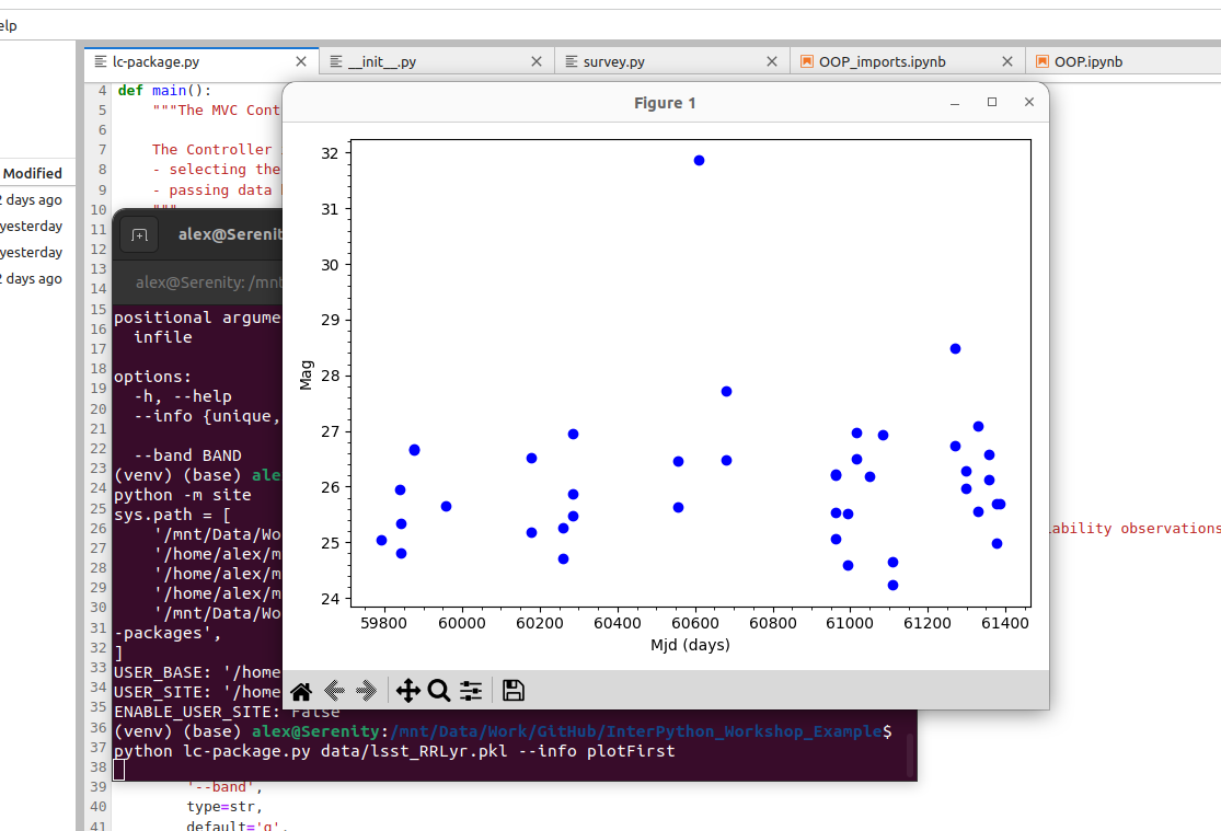
The help for the script can be accessed using the -h or --help optional argument
(which argparse includes by default):
$ python3 lc-package.py --help
usage: lc-package.py [-h] [--info {unique,plotFirst}] [--band BAND] infile

A package for inspecting LSST survey tables containing variability
observations

positional arguments:
  infile                Input CSV or PKL file containing LSST light curves

options:
  -h, --help            show this help message and exit
  --info {unique,plotFirst}
                        Which info should be displayed?
  --band BAND           Which band should be plotted?
The help page starts with the command line usage,
illustrating what inputs can be given (any within [] brackets are optional).
It then lists the positional and optional arguments,
giving as detailed a description of each as you have added to the add_argument() command.
Positional arguments are arguments that need to be included
in the proper position or order when calling the script.
Note that optional arguments are indicated by - or --, followed by the argument name.
Positional arguments are simply inferred by their position.
It is possible to have multiple positional arguments,
but usually this is only practical where all (or all but one) positional arguments
contains a clearly defined number of elements.
If more than one option can have an indeterminate number of entries,
then it is better to create them as ‘optional’ arguments.
These can be made a required input though,
by setting required = True within the add_argument() command.
Positional and Optional Argument Order
The usage section of the help page above shows the optional arguments going before the positional arguments. This is the customary way to present options, but is not mandatory. Instead there are two rules which must be followed for these arguments:
- Positional and optional arguments must each be given all together, and not inter-mixed. For example, the order can be either
optional - positionalorpositional - optional, but notoptional - positional - optional.- Positional arguments must be given in the order that they are shown in the usage section of the help page.
Optional Exercise: Add an Optional Argument For Selecting the Object
Extend our
lc-package.pycontroller by adding another optional argument that would allow the user to specify the id of the object for which they want to plot the light curve.
Towards Collaborative Software Development
Having looked at some theoretical aspects of software design, we are now circling back to developing our software to satisfy the requirements collaboratively in a team. One practice that should always be considered, and has been shown to be very effective in team-based software development, is that of code review. Code reviews help to ensure the ‘good’ coding standards are achieved and maintained within a team by having multiple people have a look and comment on key code changes to see how they fit within the codebase. Such reviews check the correctness of the new code, test coverage, functionality changes, and confirm that they follow the coding guides and best practices. Let’s have a look at some code review techniques available to us.
Key Points
By breaking down our software into components with a single responsibility, we avoid having to rewrite it all when requirements change. Such components can be as small as a single function, or be a software package in their own right.
Section 4: Collaborative Software Development for Reuse
Overview
Teaching: 5 min
Exercises: 0 minQuestions
What practices help us develop software collaboratively that will make it easier for us and others to further develop and reuse it?
Objectives
Understand the code review process and employ it to improve the quality of code.
Understand the process and best practices for preparing Python code for reuse by others.
When changes - particularly big changes - are made to a codebase, how can we as a team ensure that these changes are well considered and represent good solutions? And how can we increase the overall knowledge of a codebase across a team? Sometimes project goals and time pressures take precedence and producing maintainable, reusable code is not given the time it deserves. So, when a change or a new feature is needed - often the shortest route to making it work is taken as opposed to a more well thought-out solution. For this reason, it is important not to write the code alone and in isolation and use other team members to verify each other’s code and measure our coding standards against. This process of having multiple team members comment on key code changes is called code review - this is one of the most important practices of collaborative software development that helps ensure the ‘good’ coding standards are achieved and maintained within a team, as well as increasing knowledge about the codebase across the team. We’ll thus look at the benefits of reviewing code, in particular, the value of this type of activity within a team, and how this can fit within various ways of team working. We’ll see how GitHub can support code review activities via pull requests, and how we can do these ourselves making use of best practices.
After that, we’ll look at some general principles of software maintainability and the benefits that writing maintainable code can give you. There will also be some practice at identifying problems with existing code, and some general, established practices you can apply when writing new code or to the code you’ve already written. We’ll also look at how we can package software for release and distribution, using Poetry to manage our Python dependencies and produce a code package we can use with a Python package indexing service to illustrate these principles.
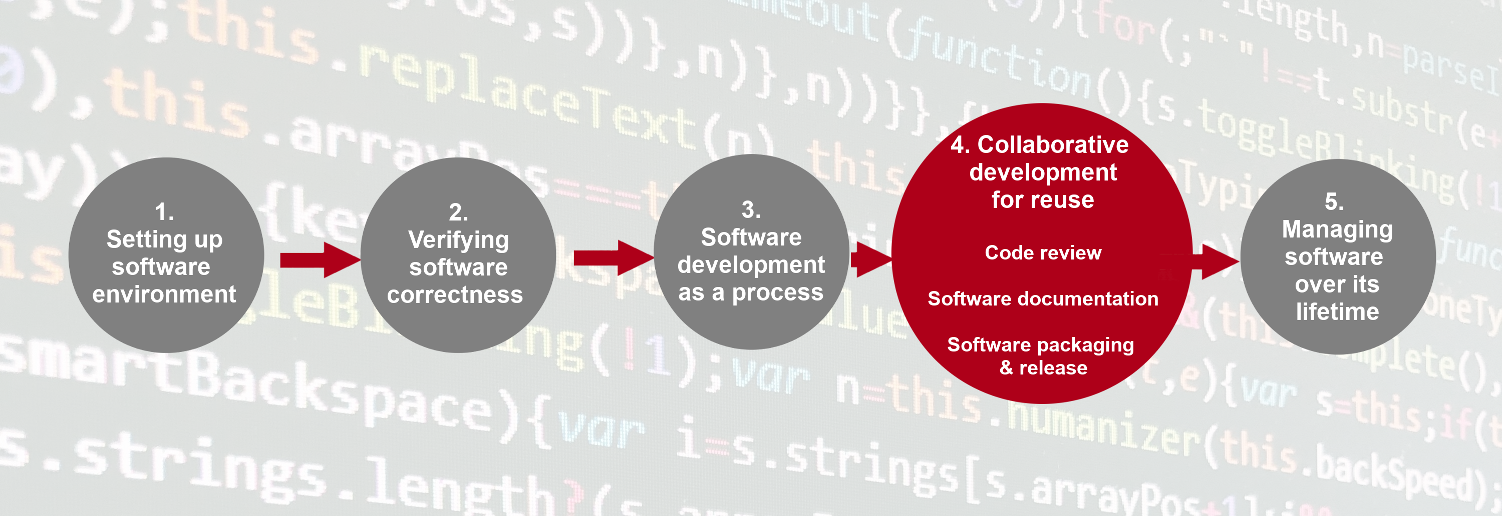
Key Points
Agreeing on a set of best practices within a software development team will help to improve your software’s understandability, extensibility, testability, reusability and overall sustainability.
Developing Software In a Team: Code Review
Overview
Teaching: 30 min
Exercises: 10 minQuestions
How do we develop software in a team?
What is code review and how it can improve the quality of code?
Objectives
Describe commonly used code review techniques.
Understand how to do a pull request via GitHub to engage in code review with a team and contribute to a shared code repository.
Introduction
So far in this course we’ve focused on learning software design and (some) technical practices, tools and infrastructure that help the development of software in a team environment, but in an individual setting. Despite developing tests to check our code - no one else from the team had a look at our code before we merged it into the main development stream. Software is often designed and built as part of a team, so in this episode we’ll be looking at how to manage the process of team software development and improve our code by engaging in code review process with other team members.
Collaborative Code Development Models
The way your team provides contributions to the shared codebase depends on the type of development model you use in your project. Two commonly used models are:
- Fork and pull model
- Shared repository model
Fork and Pull Model
In this model, anyone can fork an existing repository (to create their copy of the project linked to the source) and push changes to their personal fork. A contributor can work independently on their own fork as they do not need permissions on the source repository to push modifications to a fork they own. The changes from contributors can then be pulled into the source repository by the project maintainer on request and after a code review process. This model is popular with open source projects as it reduces the start up costs for new contributors and allows them to work independently without upfront coordination with source project maintainers. So, for example, you may use this model when you are an external collaborator on a project rather than a core team member.
Shared Repository Model
In this model, collaborators are granted push access to a single shared code repository. By default, collaborators have write access to the main branch. However, it is best practice to create feature branches for new developments, and protect the main branch. See the extra on protecting the main branch for how to do this. While it requires more upfront coordination, it is easier to share each others work, so it works well for more stable teams. This model is more prevalent with teams and organizations collaborating on private projects.
Regardless of the collaborative code development model you and your collaborators use - code reviews are one of the widely accepted best practices for software development in teams and something you should adopt in your development process too.
Code Review
Code review is a software quality assurance practice where one or several people from the team (different from the code’s author) check the software by viewing parts of its source code at the point when the code changes. Code review is very useful for all parties involved - someone checks your design or code for errors and gets to learn from your solution; having to explain code to someone else clarifies your rationale and design decisions in your mind too.
Code review is universally applicable throughout the software development cycle - from design to development to maintenance. According to Michael Fagan, the author of the code inspection technique, rigorous inspections can remove 60-90% of errors from the code even before the first tests are run (Fagan, 1976). Furthermore, according to Fagan, the cost to remedy a defect in the early (design) stage is 10 to 100 times less compared to fixing the same defect in the development and maintenance stages, respectively. Since the cost of bug fixes grows in orders of magnitude throughout the software lifecycle, it is far more efficient to find and fix defects as close as possible to the point where they were introduced.
There are several code review techniques with various degree of formality and the use of a technical infrastructure, including:
- Over-the-shoulder code review - one developer talks the other developer through the code changes while sitting at the same machine.
- Pair programming - two developers work on the code at the same time with one of them actively coding and the other providing real-time feedback.
- Formal code inspection - up to 6 partipants go through a formalised process to inspect the code specification or design for defects.
- Tool assisted code review - developers use tools such as GitHub to review the code independently and give feedback.
You can read more about these techniques in the “Five Types of Review” section of the “Best Kept Secrets of Peer Code Review” eBook.
It is worth trying multiple code review techniques to see what works best for you and your team. We will have a look at the tool-assisted code review process, which is likely to be the most effective and efficient. We will use GitHub’s built-in code review tool - pull requests, or PRs. It is a lightweight tool, included with GitHub’s core service for free and has gained popularity within the software development community in recent years.
Code Reviews via GitHub’s Pull Requests
Pull requests are fundamental to how teams review and improve code
on GitHub (and similar code sharing platforms) -
they let you tell others about changes you’ve pushed to a branch in a repository on GitHub
and that your code is ready for review.
Once a pull request is opened,
you can discuss and review the potential changes with others on the team
and add follow-up commits based on the feedback
before your changes are merged from your feature branch into the develop branch.
The name ‘pull request’ suggests you are requesting the codebase moderators
to pull your changes into the codebase.
Such changes are normally done on a feature branch,
to ensure that they are separate and self-contained,
that the main branch only contains “production-ready” work,
and that the develop branch contains code that has already been extensively tested.
You create a branch for your work based on one of the existing branches
(typically the develop branch but can be any other branch),
do some commits on that branch,
and, once you are ready to merge your changes,
create a pull request to bring the changes back to the branch that you started from.
In this context, the branch from which you branched off to do your work
and where the changes should be applied back to
is called the base branch,
while the feature branch that contains changes you would like to be applied is the head branch.
How you create your feature branches and open pull requests in GitHub will depend on your collaborative code development model:
- In the shared repository model, in order to create a feature branch and open a pull request based on it you must have write access to the source repository or, for organisation-owned repositories, you must be a member of the organisation that owns the repository. Once you have access to the repository, you proceed to create a feature branch on that repository directly.
- In the fork and pull model, where you do not have write permissions to the source repository, you need to fork the repository first before you create a feature branch (in your fork) to base your pull request on.
In both development models, it is recommended to create a feature branch for your work and the subsequent pull request, even though you can submit pull requests from any branch or commit. This is because, with a feature branch, you can push follow-up commits as a response to feedback and update your proposed changes within a self-contained bundle. The only difference in creating a pull request between the two models is how you create the feature branch. In either model, once you are ready to merge your changes in - you will need to specify the base branch and the head branch.
Code Review and Pull Requests In Action
Let’s see this in action - you and your fellow learners are going to be organised in small teams and assume to be collaborating in the shared repository model. You will be added as a collaborator to another team member’s repository (which becomes the shared repository in this context) and, likewise, you will add other team members as collaborators on your repository. You can form teams of two and work on each other’s repositories. If there are 3 members in your group you can go in a round robin fashion (the first team member does a pull request on the second member’s repository and receives a pull request on their repository from the third team member). If you are going through the material on your own and do not have a collaborator, you can do pull requests on your own repository from one to another branch.
Recall solution requirements from the last exercise in the OOP episode.
Your team member has implemented one of them according to the specification
(let’s call it feature-x)
but tests are still missing.
You are now tasked with implementing tests on top of that existing implementation
to make sure the new feature indeed satisfies the requirements.
You will propose changes to their repository
(the shared repository in this context)
via pull request (acting as the code author)
and engage in code review with your team member (acting as a code reviewer).
Similarly, you will receive a pull request on your repository from another team member,
in which case the roles will be reversed.
The following diagram depicts the branches that you should have in the repository.

Adapted from Git Tutorial by sillevl (Creative Commons Attribution 4.0 International License)
To achieve this, the following steps are needed.
Step 1: Adding Collaborators to a Shared Repository
You need to add the other team member(s) as collaborator(s) on your repository to enable them to create branches and pull requests. To do so, each repository owner needs to:
- Head over to Settings section of your software project’s repository in GitHub.

- Select the vertical tab ‘Collaborators’ from the left and click the ‘Add people’ button.

- Add your collaborator(s) by their GitHub username(s), full name(s) or email address(es).
- Collaborator(s) will be notified of your invitation to join your repository based on their notification preferences.
- Once they accept the invitation, they will have the collaborator-level access to your repository and will show up in the list of your collaborators.
See the full details on collaborator permissions for personal repositories to understand what collaborators will be able to do within your repository. Note that repositories owned by an organisation have a more granular access control compared to that of personal repositories.
Step 2: Preparing Your Local Environment for a Pull Request
- Obtain the GitHub URL of the shared repository you will be working on and clone it locally
(make sure you do it outside your software repository’s folder you have been working on so far).
This will create a copy of the repository locally on your machine
along with all of its (remote) branches.
$ git clone <remote-repo-url> $ cd <remote-repo-name> - Check with the repository owner (your team member)
which feature they implemented in the
previous exercise (it also should be stated on the top of the
.pyfiles with the corresponding classes) and what is the name of the branch they worked on. Let’s assume the name of the branch wasfeature-x(you should amend the branch name for your case accordingly). -
Your task is to add tests for the code on
feature-xbranch. You should do so on a separate branch calledfeature-x-tests, which will branch offfeature-x. This is to enable you later on to create a pull request from yourfeature-x-testsbranch with your changes that can then easily be reviewed and compared withfeature-xby the team member who created it.To do so, branch off a new local branch
feature-x-testsfrom the remotefeature-xbranch (making sure you use the branch names that match your case). Also note that, while we say “remote” branchfeature-x- you have actually obtained it locally on your machine when you cloned the remote repository.$ git checkout -b feature-x-tests origin/feature-xYou are now located in the new (local)
feature-x-testsbranch and are ready to start adding your code.
Step 3: Adding New Code
Exercise: Implement Tests for the New Feature
Look at the solution requirements for the feature that was implemented in your shared repository. Implement tests against the appropriate specification in your local feature branch.
Note: Try not to not fall into the trap of writing the tests to test the existing code/implementation - you should write the tests to make sure the code satisfies the requirements regardless of the actual implementation. You can treat the implementation as a black box - a typical approach to software testing - as a way to make sure it is properly tested against its requirements without introducing assumptions into the tests about its implementation.
Testing Based on Requirements
Tests should test functionality, which stem from the software requirements, rather than an implementation. Tests can be seen as a reflection of those requirements - checking if the requirements are satisfied.
Exercise: Edit One of the Notebooks
Comparing changes introduced to a notebook may be problematic, since notebooks aren’t plain text format. Open one of the notebooks in the
feature-x-testsbranch and make some small changes, e.g. make a plot for a different light curve from our dataset. We will use this change later.
Remember to commit your new code to your branch feature-x-tests.
$ git add -A
$ git commit -m "Added tests for feature-x."
Step 4: Submitting a Pull Request
When you have finished adding your tests
and committed the changes to your local feature-x-tests,
and are ready for the others in the team to review them,
you have to do the following:
- Push your local feature branch
feature-x-testsremotely to the shared repository.$ git push -u origin feature-x-tests - Head over to the remote repository in GitHub
and locate your new (
feature-x-tests) branch from the dropdown box on the Code tab (you can search for your branch or use the “View all branches” option).
- Open a pull request by clicking “Compare & pull request” button.
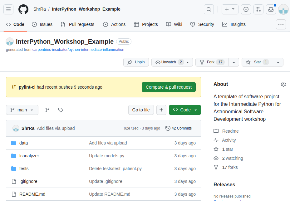
- Select the base and the head branch, e.g.
feature-xandfeature-x-tests, respectively. Recall that the base branch is where you want your changes to be merged and the head branch contains your changes. - Add a comment describing the nature of the changes, and then submit the pull request.
- Repository moderator and other collaborators on the repository (code reviewers) will be notified of your pull request by GitHub.
- At this point, the code review process is initiated.
You should receive a similar pull request from other team members on your repository.
Step 5: Code Review
- The repository moderator/code reviewers reviews your changes and provides feedback to you in the form of comments.
- Respond to their comments and do any subsequent commits, as requested by reviewers.
- It may take a few rounds of exchanging comments and discussions until the team is ready to accept your changes.
Perform the above actions on the pull request you received,
this time acting as the moderator/code reviewer.
In this role, look through the
Commits, Checks and Files tabs. They provide you with information on what
are the commits that will be merged with your branch, whether the code passed all the
workflow checks, and in case of the Files, help you to see the introduced changes in each
file, with green highlighting the additions and red highlighting what was deleted.
In the Files, pay attention to the .ipynb files (it is likely that you will need to click
on the Load diff). The changes contain a lot of cell metainformation that changes at each execution of
the cell, even if the actual output didn’t change. In order to review these changes properly, click on your
avatar in the top right corner of the window and select Feature Preview option. There in the left side
menu you can activate the Rich Jupyter Notebook Diffs that will give you an opportunity to review
the notebooks much like the ordinary .py files.
Step 6: Closing a Pull Request
- Once the moderator approves your changes, either one of you can merge onto the base branch.
Typically, it is the responsibility of the code’s author to do the merge
but this may differ from team to team.
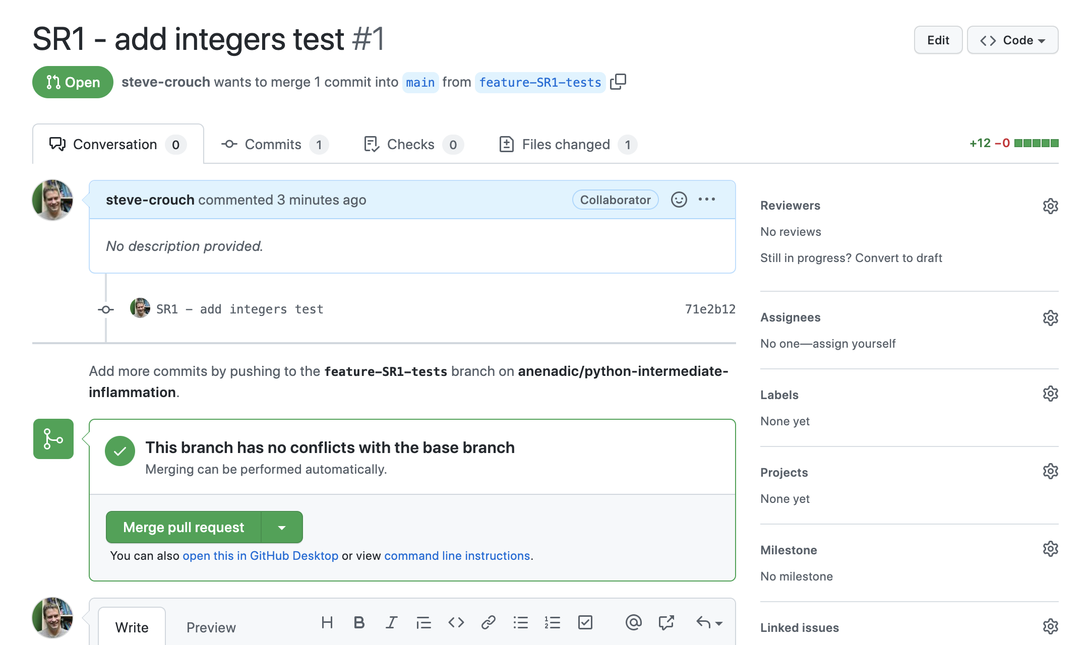
- Delete the merged branch to reduce the clutter in the repository.
Repeat the above actions for the pull request you received.
If the work on the feature branch is completed and it is sufficiently tested,
the feature branch can now be merged into the develop branch.
Best Practice for Code Review
There are multiple perspectives to a code review process - from general practices to technical details relating to different roles involved in the process. It is critical for the code’s quality, stability and maintainability that the team decides on this process and sticks to it. Here are some examples of best practices for you to consider (also check these useful code review blogs from Swarmia and Smartbear):
- Decide the focus of your code review process, e.g., consider some of the following:
- code design and functionality - does the code fit in the overall design and does it do what was intended?
- code understandability and complexity - is the code readable and would another developer be able to understand it?
- tests - does the code have automated tests?
- naming - are names used for variables and functions descriptive, do they follow naming conventions?
- comments and documentation - are there clear and useful comments that explain complex designs well and focus on the “why/because” rather than the “what/how”?
- Do not review code too quickly and do not review for too long in one sitting. According to “Best Kept Secrets of Peer Code Review” (Cohen, 2006) - the first hour of review matters the most as detection of defects significantly drops after this period. Studies into code review also show that you should not review more than 400 lines of code at a time. Conducting more frequent shorter reviews seems to be more effective.
- Decide on the level of depth for code reviews to maintain the balance between the creation time and time spent reviewing code - e.g. reserve them for critical portions of code and avoid nit-picking on small details. Try using automated checks and linters when possible, e.g. for consistent usage of certain terminology across the code and code styles.
- Communicate clearly and effectively - when reviewing code, be explicit about the action you request from the author.
- Foster a positive feedback culture:
- give feedback about the code, not about the author
- accept that there are multiple correct solutions to a problem
- sandwich criticism with positive comments and praise
- Utilise multiple code review techniques - use email, pair programming, over-the-shoulder, team discussions and tool-assisted or any combination that works for your team. However, for the most effective and efficient code reviews, tool-assisted process is recommended.
- From a more technical perspective:
- use a feature branch for pull requests as you can push follow-up commits if you need to update your proposed changes
- avoid large pull requests as they are more difficult to review. You can refer to some studies and Google recommendations as to what a “large pull request” is but be aware that it is not exact science.
- don’t force push to a pull request as it changes the repository history and can corrupt your pull request for other collaborators.
Exercise: Code Review in Your Own Working Environment
At the start of this episode we briefly looked at a number of techniques for doing code review, and as an example, went on to see how we can use GitHub Pull Requests to review team member code changes. Finally, we also looked at some best practices for doing code reviews in general.
Now think about how you typically develop code, and how you might institute code review practices within your own working environment. Discuss in your group with whom among your peers of collegues you could team up for the code review. Think about the possibilites to introduce this practice to the programming courses in your university or make it a part of the weekly group meeting. Which code review approaches would be the most practical for you?
Key Points
Code review is a team software quality assurance practice where team members look at parts of the codebase in order to improve their code’s readability, understandability, quality and maintainability.
It is important to agree on a set of best practices and establish a code review process in a team to help to sustain a good, stable and maintainable code for many years.
Preparing Software for Reuse and Release
Overview
Teaching: 35 min
Exercises: 20 minQuestions
What can we do to make our programs reusable by others?
How should we document and license our code?
Objectives
Describe the different levels of software reusability
Explain why documentation is important
Describe the minimum components of software documentation to aid reuse
Create a repository README file to guide others to successfully reuse a program
Understand other documentation components and where they are useful
Describe the basic types of open source software licence
Explain the importance of conforming to data policy and regulation
Prioritise and work on improvements for release as a team
Introduction
In previous episodes we’ve looked at skills, practices, and tools to help us design and develop software in a collaborative environment. In this lesson we’ll be looking at a critical piece of the development puzzle that builds on what we’ve learnt so far - sharing our software with others.
The Levels of Software Reusability - Good Practice Revisited
Let’s begin by taking a closer look at software reusability and what we want from it.
Firstly, whilst we want to ensure our software is reusable by others, as well as ourselves, we should be clear what we mean by ‘reusable’. There are a number of definitions out there, but a helpful one written by Benureau and Rougler in 2017 offers the following levels by which software can be characterised:
- Re-runnable: the code is simply executable and can be run again (but there are no guarantees beyond that)
- Repeatable: the software will produce the same result more than once
- Reproducible: published research results generated from the same version of the software can be generated again from the same input data
- Reusable: easy to use, understand, and modify
- Replicable: the software can act as an available reference for any ambiguity in the algorithmic descriptions made in the published article. That is, a new implementation can be created from the descriptions in the article that provide the same results as the original implementation, and that the original - or reference - implementation, can be used to clarify any ambiguity in those descriptions for the purposes of reimplementation
Later levels imply the earlier ones. So what should we aim for? As researchers who develop software - or developers who write research software - we should be aiming for at least the fourth one: reusability. Reproducibility is required if we are to successfully claim that what we are doing when we write software fits within acceptable scientific practice, but it is also crucial that we can write software that can be understood and ideally modified by others. If others are unable to verify that a piece of software follows published algorithms, how can they be certain it is producing correct results? Where ‘others’, of course, can include a future version of ourselves.
Documenting Code to Improve Reusability
Reproducibility is a cornerstone of science, and scientists who work in many disciplines are expected to document the processes by which they’ve conducted their research so it can be reproduced by others. In medicinal, pharmacological, and similar research fields for example, researchers use logbooks which are then used to write up protocols and methods for publication.
Many things we’ve covered so far contribute directly to making our software reproducible - and indeed reusable - by others. A key part of this we’ll cover now is software documentation, which is ironically very often given short shrift in academia. This is often the case even in fields where the documentation and publication of research method is otherwise taken very seriously.
A few reasons for this are that writing documentation is often considered:
- A low priority compared to actual research (if it’s even considered at all)
- Expensive in terms of effort, with little reward
- Writing documentation is boring!
A very useful form of documentation for understanding our code is code commenting, and is most effective when used to explain complex interfaces or behaviour, or the reasoning behind why something is coded a certain way. But code comments only go so far.
Whilst it’s certainly arguable that writing documentation isn’t as exciting as writing code, it doesn’t have to be expensive and brings many benefits. In addition to enabling general reproducibility by others, documentation…
- Helps bring new staff researchers and developers up to speed quickly with using the software
- Functions as a great aid to research collaborations involving software, where those from other teams need to use it
- When well written, can act as a basis for detailing algorithms and other mechanisms in research papers, such that the software’s functionality can be replicated and re-implemented elsewhere
- Provides a descriptive link back to the science that underlies it. As a reference, it makes it far easier to know how to update the software as the scientific theory changes (and potentially vice versa)
- Importantly, it can enable others to understand the software sufficiently to modify and reuse it to do different things
In the next section we’ll see that writing a sensible minimum set of documentation in a single document doesn’t have to be expensive, and can greatly aid reproducibility.
Writing a README
A README file is the first piece of documentation (perhaps other than publications that refer to it) that people should read to acquaint themselves with the software. It concisely explains what the software is about and what it’s for, and covers the steps necessary to obtain and install the software and use it to accomplish basic tasks. Think of it not as a comprehensive reference of all functionality, but more a short tutorial with links to further information - hence it should contain brief explanations and be focused on instructional steps.
Our repository already has a README that describes the purpose of the repository for this workshop, but let’s replace it with a new one that describes the software itself. First let’s delete the old one:
$ rm README.md
In the root of your repository create a replacement README.md file.
The .md indicates this is a Markdown file,
a lightweight markup language which is basically a text file with
some extra syntax to provide ways of formatting them.
A big advantage of them is that they can be read as plain-text files
or as source files for rendering them with formatting structures,
and are very quick to write.
GitHub provides a very useful guide to writing Markdown for its repositories.
Let’s start writing README.md using a text editor of your choice and add the following line.
# LcAnalyzer
So here, we’re giving our software a name.
Ideally something unique, short, snappy, and perhaps to some degree an indicator of what it does.
We would ideally rename the repository to reflect the new name, but let’s leave that for now.
In Markdown, the # designates a heading, two ## are used for a subheading, and so on.
The Software Sustainability Institute’s
guide on naming projects
and products provides some helpful pointers.
We should also add a short description underneath the title.
# LcAnalyzer
LcAnalyzer is a package written in Python that allows you to inspect light curves.
To give readers an idea of the software’s capabilities, let’s add some key features next:
# LcAnalyzer
LcAnalyzer is a package written in Python that allows you to inspect light curves.

## Main features
Here are some key features of LcAnalyzer:

- Reading CSV and Pickle files;
- Giving the list of unique objects present in the data;
- Selecting observations of a given star in a given bands;
...
As well as knowing what the software aims to do and its key features,
it’s very important to specify what other software and related dependencies
are needed to use the software (typically called dependencies or prerequisites):
...

## Prerequisites
LcAnalyzer requires the following Python packages:

- [Pandas](https://pandas.pydata.org/) - makes use of Pandas's data types and statistical functions
- [Matplotlib](https://matplotlib.org/stable/index.html) - uses Matplotlib to generate statistical plots

The following optional packages are required to run LcAnalyzer's unit tests:

- [pytest](https://docs.pytest.org/en/stable/) - LcAnalyzer's unit tests are written using pytest
- [pytest-cov](https://pypi.org/project/pytest-cov/) - Adds test coverage stats to unit testing
Here we’re making use of Markdown links,
with some text describing the link within [] followed by the link itself within ().
One really neat feature - and a common practice - of using many CI infrastructures is that
we can include the status of running recent tests within our README file.
Just below the # LcAnalyzer title on our README.md file,
add the following (replacing <your_github_username> with your own:
# LcAnalyzer

...
This will embed a badge (icon) at the top of our page that
reflects the most recent GitHub Actions build status of your software repository,
essentially showing whether the tests that were run
when the last change was made to the main branch succeeded or failed.
That’s got us started with documenting our code, but there are other aspects we should also cover:
- Installation/deployment: step-by-step instructions for setting up the software so it can be used
- Basic usage: step-by-step instructions that cover using the software to accomplish basic tasks
- Contributing: for those wishing to contribute to the software’s development, this is an opportunity to detail what kinds of contribution are sought and how to get involved
- Contact information/getting help: which may include things like key author email addresses, and links to mailing lists and other resources
- Credits/acknowledgements: where appropriate, be sure to credit those who have helped in the software’s development or inspired it
- Citation: particularly for academic software, it’s a very good idea to specify a reference to an appropriate academic publication so other academics can cite use of the software in their own publications and media. You can do this within a separate CITATION text file within the repository’s root directory and link to it from the Markdown
- Licence: a short description of and link to the software’s licence
For more verbose sections, there are usually just highlights in the README with links to further information, which may be held within other Markdown files within the repository or elsewhere.
We’ll finish these off later. See Matias Singer’s curated list of awesome READMEs for inspiration.
Other Documentation
There are many different types of other documentation you should also consider writing and making available that’s beyond the scope of this course. The key is to consider which audiences you need to write for, e.g. end users, developers, maintainers, etc., and what they need from the documentation. There’s a Software Sustainability Institute blog post on best practices for research software documentation that helpfully covers the kinds of documentation to consider and other effective ways to convey the same information.
One that you should always consider is technical documentation. This typically aims to help other developers understand your code sufficiently well to make their own changes to it, including external developers, other members in your team and a future version of yourself too. This may include documentation that covers the software’s architecture, including its different components and how they fit together, API (Application Programming Interface) documentation that describes the interface points designed into your software for other developers to use, e.g. for a software library, or technical tutorials/’HOW TOs’ to accomplish developer-oriented tasks.
Choosing an Open Source Licence
Software licensing is a whole topic in itself, so we’ll just summarise here. Your institution’s Intellectual Property (IP) team will be able to offer specific guidance that fits the way your institution thinks about software.
In IP law, software is considered a creative work of literature, so any code you write automatically has copyright protection applied. This copyright will usually belong to the institution that employs you, but this may be different for PhD students. If you need to check, this should be included in your employment/studentship contract or talk to your university’s IP team.
Since software is automatically under copyright, without a licence no one may:
- Copy it
- Distribute it
- Modify it
- Extend it
- Use it (actually unclear at present - this has not been properly tested in court yet)
Fundamentally there are two kinds of licence, Open Source licences and Proprietary licences, which serve slightly different purposes:
- Proprietary licences are designed to pass on limited rights to end users, and are most suitable if you want to commercialise your software. They tend to be customised to suit the requirements of the software and the institution to which it belongs - again your institutions IP team will be able to help here.
- Open Source licences are designed more to protect the rights of end users - they specifically grant permission to make modifications and redistribute the software to others. The website Choose A License provides recommendations and a simple summary of some of the most common open source licences.
Within the open source licences, there are two categories, copyleft and permissive:
- The permissive licences such as MIT and the multiple variants of the BSD licence are designed to give maximum freedom to the end users of software. These licences allow the end user to do almost anything with the source code.
- The copyleft licences in the GPL still give a lot of freedom to the end users, but any code that they write based on GPLed code must also be licensed under the same licence. This gives the developer assurance that anyone building on their code is also contributing back to the community. It’s actually a little more complicated than this, and the variants all have slightly different conditions and applicability, but this is the core of the licence.
Which of these types of licence you prefer is up to you and those you develop code with. If you want more information, or help choosing a licence, the Choose An Open-Source Licence or tl;dr Legal sites can help.
Exercise: Preparing for Release
In a (hopefully) highly unlikely and thoroughly unrecommended scenario, your project leader has informed you of the need to release your software within the next half hour, so it can be assessed for use by another team. You’ll need to consider finishing the README, choosing a licence, and fixing any remaining problems you are aware of in your codebase. Ensure you prioritise and work on the most pressing issues first!
Merging into main
Once you’ve done these updates,
commit your changes,
and if you’re doing this work on a feature branch also ensure you merge it into develop,
e.g.:
$ git checkout develop
$ git merge my-feature-branch
Finally, once we’ve fully tested our software
and are confident it works as expected on develop,
we can merge our develop branch into main:
$ git checkout main
$ git merge develop
$ git push
Tagging a Release in GitHub
There are many ways in which Git and GitHub can help us make a software release from our code. One of these is via tagging, where we attach a human-readable label to a specific commit. Let’s see what tags we currently have in our repository:
$ git tag
Since we haven’t tagged any commits yet, there’s unsurprisingly no output. We can create a new tag on the last commit we did by doing:
$ git tag -a v1.0.0 -m "Version 1.0.0"
So we can now do:
$ git tag
v.1.0.0
And also, for more information:
$ git show v1.0.0
You should see something like this:
tag v1.0.0
Tagger: <Name> <email>
Date:   Fri Dec 10 10:22:36 2021 +0000

Version 1.0.0

commit 2df4bfcbfc1429c12f92cecba751fb2d7c1a4e28 (HEAD -> main, tag: v1.0.0, origin/main, origin/develop, origin/HEAD, develop)
Author: <Name> <email>
Date:   Fri Dec 10 10:21:24 2021 +0000

	Finalising README.

diff --git a/README.md b/README.md
index 4818abb..5b8e7fd 100644
--- a/README.md
+++ b/README.md
@@ -22,4 +22,33 @@ Flimflam requires the following Python packages:
 The following optional packages are required to run Flimflam's unit tests:

 - [pytest](https://docs.pytest.org/en/stable/) - Flimflam's unit tests are written using pytest
-- [pytest-cov](https://pypi.org/project/pytest-cov/) - Adds test coverage stats to unit testing
\ No newline at end of file
+- [pytest-cov](https://pypi.org/project/pytest-cov/) - Adds test coverage stats to unit testing
+
+## Installation
+- Clone the repo ``git clone repo``
+- Check everything runs by running ``python -m pytest`` in the root directory
+- Hurray 😊
+
+## Contributing
+- Create an issue [here](https://github.com/Onoddil/python-intermediate-inflammation/issues)
+  - What works, what doesn't? You tell me
+- Randomly edit some code and see if it improves things, then submit a [pull request](https://github.com/Onoddil/python-intermediate-inflammation/pulls)
+- Just yell at me while I edit the code, pair programmer style!
+
+## Getting Help
+- Nice try
+
+## Credits
+- Directed by Michael Bay
+
+## Citation
+Please cite [J. F. W. Herschel, 1829, MmRAS, 3, 177](https://ui.adsabs.harvard.edu/abs/1829MmRAS...3..177H/abstract) if you used this work in your day-to-day life.
+Please cite [C. Herschel, 1787, RSPT, 77, 1](https://ui.adsabs.harvard.edu/abs/1787RSPT...77....1H/abstract) if you actually use this for scientific work.
+
+## License
+This source code is protected under international copyright law.  All rights
+reserved and protected by the copyright holders.
+This file is confidential and only available to authorized individuals with the
+permission of the copyright holders.  If you encounter this file and do not have
+permission, please contact the copyright holders and delete this file.
\ No newline at end of file
So now we’ve added a tag, we need this reflected in our Github repository. You can push this tag to your remote by doing:
$ git push origin v1.0.0
What is a Version Number Anyway?
Software version numbers are everywhere, and there are many different ways to do it. A popular one to consider is Semantic Versioning, where a given version number uses the format MAJOR.MINOR.PATCH. You increment the:
- MAJOR version when you make incompatible API changes
- MINOR version when you add functionality in a backwards compatible manner
- PATCH version when you make backwards compatible bug fixes
You can also add a hyphen followed by characters to denote a pre-release version, e.g. 1.0.0-alpha1 (first alpha release) or 1.2.3-beta4 (fourth beta release)
We can now use the more memorable tag to refer to this specific commit.
Plus, once we’ve pushed this back up to GitHub,
it appears as a specific release within our code repository
which can be downloaded in compressed .zip or .tar.gz formats.
Note that these downloads just contain the state of the repository at that commit,
and not its entire history.
Using features like tagging allows us to highlight commits that are particularly important, which is very useful for reproducibility purposes. We can (and should) refer to specific commits for software in academic papers that make use of results from software, but tagging with a specific version number makes that just a little bit easier for humans.
Conforming to Data Policy and Regulation
We may also wish to make data available to either be used with the software or as generated results. This may be via GitHub or some other means. An important aspect to remember with sharing data on such systems is that they may reside in other countries, and we must be careful depending on the nature of the data.
We need to ensure that we are still conforming to the relevant policies and guidelines regarding how we manage research data, which may include funding council, institutional, national, and even international policies and laws. Within Europe, for example, there’s the need to conform to things like GDPR. It’s a very good idea to make yourself aware of these aspects.
Key Points
The reuse battle is won before it is fought. Select and use good practices consistently throughout development and not just at the end.
Packaging Code for Release and Distribution
Overview
Teaching: 0 min
Exercises: 20 minQuestions
How do we prepare our code for sharing as a Python package?
How do we release our project for other people to install and reuse?
Objectives
Describe the steps necessary for sharing Python code as installable packages.
Use Poetry to prepare an installable package.
Explain the differences between runtime and development dependencies.
Why Package our Software?
We’ve now got our software ready to release - the last step is to package it up so that it can be distributed.
For very small pieces of software, for example a single source file, it may be appropriate to distribute to non-technical end-users as source code, but in most cases we want to bundle our application or library into a package. A package is typically a single file which contains within it our software and some metadata allows it to be installed and used more simply - e.g. a list of dependencies. By distributing our code as a package, we reduce the complexity of fetching, installing and integrating it for the end-users.
In this session we’ll introduce one widely used method for building an installable package from our code. There are range of methods in common use, so it’s likely you’ll also encounter projects take different approaches.
There’s some confusing terminology in this episode around the use of the term “package”. This term is used to refer to both:
- A directory containing Python files / modules and an
__init__.py- a “module package” - A way of structuring / bundling a project for easier distribution and installation - a “distributable package”
Creating the init.py file
In order to consider a directory with .py files a package, Python requires that this directory
contained a __init__.py file. In the simplest case it can be empty (like the __init__.py in our original
lcanalyzer directory), however, it may also contain the code that will be executed when
the package is imported into another script for the first time. Often __init__.py
contains a docstring, a variable __all__ that represents a list of all methods that
should be imported when the user invokes from package_name import * statement,
a list of hard dependencies that must be imported in order for the package to be minimally functional,
different kinds of configurations (e.g. defining some specific paths) and so on.
For now we will limit ourselves to the empty __init__.py file. Create it
in the lcanalyzer directory, and make sure to commit it to the repository.
Packaging our Software with Poetry
Installing Poetry
Because we’ve recommended GitBash if you’re using Windows, we’re going to install Poetry using a different method to the officially recommended one. If you’re on MacOS or Linux, are comfortable with installing software at the command line and want to use Poetry to manage multiple projects, you may instead prefer to follow the official Poetry installation instructions.
We can install Poetry much like any other Python distributable package, using pip:
$ source venv/bin/activate
$ pip3 install poetry
To test, we can ask where Poetry is installed:
$ which poetry
/mnt/Data/Work/GitHub/InterPython_Workshop_Example/venv/bin/poetry
or what version of the package is available:
$ poetry --version
Poetry (version 1.8.3)
If you don’t get similar output, make sure you’ve got the correct virtual environment activated.
Poetry can also handle virtual environments for us, so in order to behave similarly to how we used them previously, let’s change the Poetry config to put them in the same directory as our project:
$ poetry config virtualenvs.in-project true
Setting up our Poetry Config
Poetry uses a pyproject.toml file to describe the build system and requirements of the distributable package. This file format was introduced to solve problems with bootstrapping packages (the processing we do to prepare to process something) using the older convention with setup.py files and to support a wider range of build tools. It is described in PEP 518 (Specifying Minimum Build System Requirements for Python Projects).
Make sure you are in the root directory of your software project and have activated your virtual environment, then we’re ready to begin.
To create a pyproject.toml file for our code, we can use poetry init.
This will guide us through the most important settings -
for each prompt, we either enter our data or accept the default.
Displayed below are the questions you should see with the recommended responses to each question so try to follow these, although use your own contact details!
NB: When you get to the questions about defining our dependencies, answer no, so we can do this separately later.
$ poetry init
This command will guide you through creating your pyproject.toml config.

Package name [example]:  lcanalyzer
Version [0.1.0]: 1.0.0
Description []:  Inspect light curves
Author [None, n to skip]: James Graham <J.Graham@software.ac.uk>
License []:  MIT
Compatible Python versions [^3.11]: ^3.11

Would you like to define your main dependencies interactively? (yes/no) [yes] no
Would you like to define your development dependencies interactively? (yes/no) [yes] no
Generated file

[tool.poetry]
name = "lcanalyzer"
version = "1.0.0"
description = "Inspect light curves"
authors = ["ShrRa"]
license = "MIT"
readme = "README.md"

[tool.poetry.dependencies]
python = "^3.11"


[build-system]
requires = ["poetry-core"]
build-backend = "poetry.core.masonry.api"


Do you confirm generation? (yes/no) [yes] yes
We’ve called our package “lcanalyzer” in the setup above, because Poetry will automatically find our code if the name of the distributable package matches the name of our module package. If we wanted our distributable package to have a different name, for example “lcanalysis”, we could do this by explicitly listing the module packages to bundle - see the Poetry docs on packages for how to do this.
Project Dependencies
Previously, we looked at using a requirements.txt file to define the dependencies of our software.
Here, Poetry takes inspiration from package managers in other languages,
particularly NPM (Node Package Manager),
often used for JavaScript development.
Tools like Poetry and NPM understand that there are two different types of dependency:
runtime dependencies and development dependencies.
Runtime dependencies are those dependencies that
need to be installed for our code to run, like NumPy.
Development dependencies are dependencies which
are an essential part of your development process for a project,
but are not required to run it.
Common examples of developments dependencies are linters and test frameworks,
like pylint or pytest.
When we add a dependency using Poetry,
Poetry will add it to the list of dependencies in the pyproject.toml file,
add a reference to it in a new poetry.lock file,
and automatically install the package into our virtual environment.
If we don’t yet have a virtual environment activated,
Poetry will create it for us - using the name .venv,
so it appears hidden unless we do ls -a.
Because we’ve already activated a virtual environment, Poetry will use ours instead.
The pyproject.toml file has two separate lists,
allowing us to distinguish between runtime and development dependencies.
$ poetry add matplotlib pandas
$ poetry add --group dev pylint
$ poetry install
These two sets of dependencies will be used in different circumstances.
When we build our package and upload it to a package repository,
Poetry will only include references to our runtime dependencies.
This is because someone installing our software through a tool like pip is only using it,
but probably doesn’t intend to contribute to the development of our software
and does not require development dependencies.
In contrast, if someone downloads our code from GitHub,
together with our pyproject.toml,
and installs the project that way,
they will get both our runtime and development dependencies.
If someone is downloading our source code,
that suggests that they intend to contribute to the development,
so they’ll need all of our development tools.
Have a look at the pyproject.toml file again to see what’s changed.
Packaging Our Code
The final preparation we need to do is to
make sure that our code is organised in the recommended structure.
This is the Python module structure -
a directory containing an __init__.py and our Python source code files.
Make sure that the name of this Python package
(lcanalyzer - unless you’ve renamed it)
matches the name of your distributable package in pyproject.toml
unless you’ve chosen to explicitly list the module packages.
By convention distributable package names use hyphens, whereas module package names use underscores. While we could choose to use underscores in a distributable package name, we cannot use hyphens in a module package name, as Python will interpret them as a minus sign in our code when we try to import them.
Once we’ve got our pyproject.toml configuration done and our project is in the right structure,
we can go ahead and build a distributable version of our software:
$ poetry build
This should produce two files for us in the dist directory.
The one we care most about is the .whl or wheel file.
This is the file that pip uses to distribute and install Python packages,
so this is the file we’d need to share with other people who want to install our software.
Now if we gave this wheel file to someone else,
they could install it using pip -
you don’t need to run this command yourself,
you’ve already installed it using poetry install above.
$ pip3 install dist/lcanalyzer*.whl
The star in the line above is a wildcard,
that means Bash should use any filenames that match that pattern,
with any number of characters in place for the star.
We could also rely on Bash’s autocomplete functionality and type dist/lcanalyzer,
then hit the Tab key if we’ve only got one version built.
After we’ve been working on our code for a while and want to publish an update,
we just need to update the version number in the pyproject.toml file
(using SemVer perhaps),
then use Poetry to build and publish the new version.
If we don’t increment the version number,
people might end up using this version,
even though they thought they were using the previous one.
Any re-publishing of the package, no matter how small the changes,
needs to come with a new version number.
The advantage of SemVer is that the change in the version number
indicates the degree of change in the code and thus the degree of risk of breakage when we update.
In addition to the commands we’ve already seen, Poetry contains a few more that can be useful for our development process. For the full list see the Poetry CLI documentation.
The final step is to publish our package to a package repository. A package repository could be either public or private - while you may at times be working on public projects, it’s likely the majority of your work will be published internally using a private repository such as JFrog Artifactory. Every repository may be configured slightly differently, so we’ll leave that to you to investigate.
What if We Need More Control?
Sometimes we need more control over the process of building our distributable package than Poetry allows. There many ways to distribute Python code in packages, with some degree of flux in terms of which methods are most popular. For a more comprehensive overview of Python packaging you can see the Python docs on packaging, which contains a helpful guide to the overall packaging process, or ‘flow’, using the Twine tool to upload created packages to PyPI for distribution as an alternative.
Optional Exercise: Enhancing our Package Metadata
The Python Packaging User Guide provides documentation on how to package a project using a manual approach to building a
pyproject.tomlfile, and using Twine to upload the distribution packages to PyPI.Referring to the section on metadata in the documentation, enhance your
pyproject.tomlwith some additional metadata fields to improve the information your package.
Key Points
Poetry allows us to produce an installable package and upload it to a package repository.
Making our software installable with Pip makes it easier for others to start using it.
For complete control over building a package, we can use a
setup.pyfile.
Wrap-up
Overview
Teaching: 15 min
Exercises: 0 minQuestions
Looking back at what was covered and how different pieces fit together
Where are some advanced topics and further reading available?
Objectives
Put the course in context with future learning.
Summary
As part of this course we have looked at a core set of established, intermediate-level software development tools and best practices for working as part of a team. The course teaches a selected subset of skills that have been tried and tested in collaborative research software development environments, although not an all-encompassing set of every skill you might need (check some further reading). It will provide you with a solid basis for writing industry-grade code, which relies on the same best practices taught in this course:
- Collaborative techniques and tools play an important part of research software development in teams, but also have benefits in solo development. We’ve looked at the benefits of a well-considered development environment, using practices, tools and infrastructure to help us write code more effectively in collaboration with others.
- We’ve looked at the importance of being able to verify the correctness of software and automation, and how we can leverage techniques and infrastructure to automate and scale tasks such as testing to save us time - but automation has a role beyond simply testing: what else can you automate that would save you even more time? Once found, we’ve also examined how to locate faults in our software.
- We’ve gone beyond procedural programming and explored different software design paradigms, such as object-oriented and functional styles of programming. We’ve contrasted their pros, cons, and the situations in which they work best, and how separation of concerns through modularity and architectural design can help shape good software.
- As an intermediate developer, aspects other than technical skills become important, particularly in development teams. We’ve looked at the importance of good, consistent practices for team working, and the importance of having a self-critical mindset when developing software, and ways to manage feedback effectively and efficiently.
Reflection Exercise: Putting the Pieces Together
As a group, reflect on the concepts (e.g. tools, techniques and practices) covered throughout the course, how they relate to one another, how they fit together in a bigger picture or skill learning pathways and in which order you need to learn them.
Solution
One way to think about these concepts is to make a list and try to organise them along two axes - ‘perceived usefulness of a concept’ versus ‘perceived difficulty or time needed to master a concept’, as shown in the table below (for the exercise, you can make your own copy of the template table for the purpose of this exercise). You then may think in which order you want to learn the skills and how much effort they require - e.g. start with those that are more useful but, for the time being, hold off those that are not too useful to you and take loads of time to master. You will likely want to focus on the concepts in the top right corner of the table first, but investing time to master more difficult concepts may pay off in the long run by saving you time and effort and helping reduce technical debt.
Another way you can organise the concepts is using a concept map (a directed graph depicting suggested relationships between concepts) or any other diagram/visual aid of your choice. Below are some example views of tools and techniques covered in the course using concept maps. Your views may differ but that is not to say that either view is right or wrong. This exercise is meant to get you to reflect on what was covered in the course and hopefully to reinforce the ideas and concepts you learned.
A different concept map tries to organise concepts/skills based on their level of difficulty (novice, intermediate and advanced, and in-between!) and tries to show which skills are prerequisite for others and in which order you should consider learning skills.
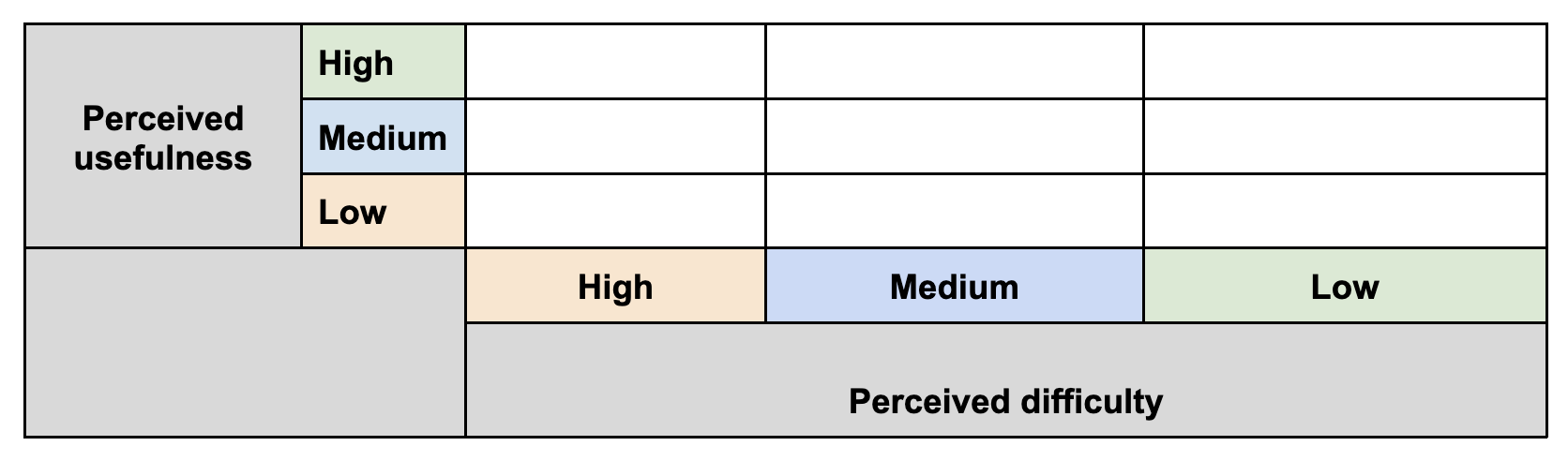
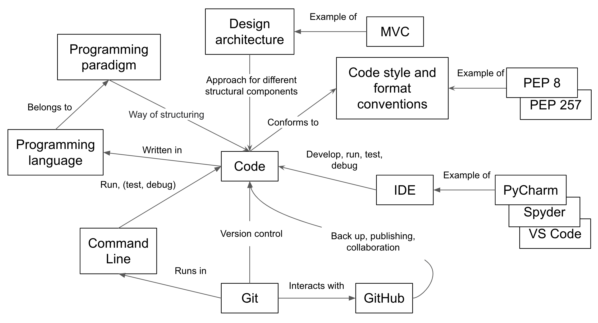
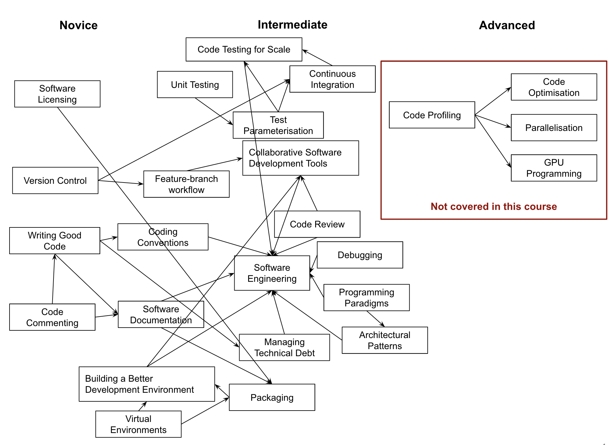
Further Resources
Below are some additional resources to help you continue learning:
- Additional episode on persisting data
- Additional episode on databases
- CodeRefinery courses on FAIR (Findable, Accessible, Interoperable, and Reusable) software practices
- Python documentation
- GitHub Actions documentation
Key Points
Collaborative techniques and tools play an important part of research software development in teams.